
STATISTICAL MODELING OF MULTIVARIATE RELIABILITY FUNCTION USING COPULA METHOD IN THE PRESENCE OF CENSORING
Abstract
Numerous scientific and practical researches conducted around the world are mostly focused use on the methods of statistical modeling. Statistical models play an impor-tant role in various fields. Examples include mathematical models in the physics, astronomy, biology, medicine, economics, demography, sociology, psychology, marketing, political science, engineering sciences, machine learning, computer science, natural sciences and other related fields. In this article, we investigate the problem of statistical modeling of multivariate reliability functions. In this case, an algorithm for constructing a statistical model is developed and the copula method is used in the presence of censoring.
Keywords and phrases: Statistical modeling, censoring, copula method, reliability function, dependent variables.
MSC 2010 Classifications: Primary 62G05; Secondary 62G20.
1. Introduction
Statistical modeling is the use of mathematical models and statistical assumptions to generate sample data and make predictions about the real world. A statistical model is a collection of probability distributions on a set of all possible outcomes of an experiment. The nonparametric estimation of a multivariate reliability function will not usually be the end-point of a statistical analysis, but it can play a crucial role in model building and testing on the way to a definitive analysis. Data analysis goals may include estimation of the failure time distribution, and study of dependencies of failure times on study subject characteristics, exposures, or treatments, gener-ically referred to as covariates. Failure time methods have application in many subject matter and research areas, including biomedical, behavioral, physical, and engineering sciences, and various industrial settings (see, [1]).
The joint distribution of a set of random variables X1, X2, ..., Xn is defined as
F(x1, x2, ..., xn) = P(X1 ≤ x1, X2 ≤ x2, ..., Xn ≤ xn),
and the reliability function corresponding to F(x1, x2, ..., xn) is given by
R(x1, x2, ..., xn) = P(X1 > x1, X2 > x2, ..., Xn > xn).
The reliability function is fundamental to a reliability theory, because obtaining reliability prob-abilities for different values of x provides crucial summary information from reliability data. For n = 1, R(x) = 1 − F(x),
for n = 2 R(x1, x2) = 1 − F1(x1) − F2(x2) + F1(x1) · F2(x2).
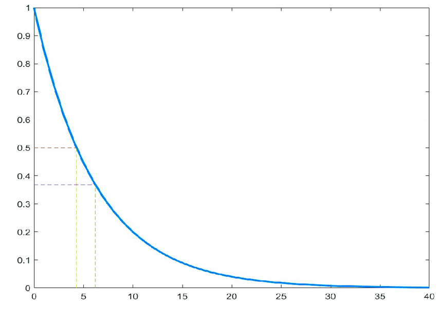
Example. For the exponential distribution, which is commonly used to model the time until an event occurs in a process with a constant failure rate, the reliability function can be defined as (see, figure 1):
R(x) = e , λ-the item failure rate under the specified operating conditions of temperature, stress, envi-ronment, etc.. This formula indicates that the reliability decreases exponentially with time x. As time increases, the probability of the system surviving beyond that time decreases. There-fore, the reliability function is simply the complement of the cumulative distribution function
−λx
F(x) = 1 − e , representing the probability that the event occurs after time x.
2. Copula method in statistical modeling
Learning and using copulas in statistical modeling is a fairly modern method (see, figure 2). By definition, copulas are parametric multivariate distributions generated from uniformly distributed marginals on a given interval [0, 1] (see, [2]). Therefore, the properties of copulas are analogous to the properties of joint distributions.
It is known that the multivariate Poisson distribution, exponential distribution or normal dis-tribution, can be considered as a good model for estimating the joint distribution of abounding microeconomic, macroeconomic and financial variables. But sometimes these distributions may not give good results. This leads to the problem of finding multivariate models that best fit this distribution. One possible way to solve this problem is to use the theory of functions known as copulas. The word copula comes from the Latin for "link" or "tie" together, where the term is used in linguistics to describe such linking words or phrases. The scientific work of mathemati-cians Hoeffding (1940) and Sklar (1959) played an important role in the initial formation of the theory of these functions (see, [2]-[11]). By the end of the 1990s, the attention of specialists was attracted by mathematical modeling using copula functions and their practical application. The copula function method consists of forming a correlation structure by connecting the marginal distributions to the joint distribution using another auxiliary link function. The use of this method is one of the current problems. The copula methodology separates marginal distributions from the dependence structure, linking them to the joint distribution through the copula function. Early monographs on copulas are Joe (1997) (with focus on novel probabilistic notions around copulas) and Nelsen (1999, 2006) (a well-known, readable introduction). An interesting histor-ical perspective and introduction can be found in Durante and Sempi (2010). A more advanced probabilistic treatment of copulas is the recent Durante and Sempi (2015). Now a days, copula functions are successfully used in finance and insurance, biostatistics (Lambert, Vandenhende, 2002)), hydrology (Zhang, Singh, 2006)) and climatology (Salvadori, De Michele, 2007)(see for detail [29]-[33]).
Let us give the definition of the two-dimensional copula function in order to understand its meaning in more detail.
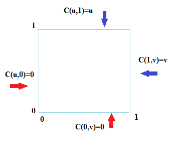
Definition 2.1. (Axiomatical) A two-dimensional copula C is a mapping from I = [0, 1]×[0, 1] to I = [0, 1] which satisfies the following three conditions:
1.(Limitation) C(u, 0) = C(0, u) = 0 for every u, v ∈ [0, 1]; 2. C(u, 1) = u, C(1, v) = v for every u, v ∈ [0, 1] (see, figure 3); 3. (Monotonicity) C(u2, v2) − C(u1, v2) − C(u2, v1) + C(u1, v1) ≥ 0 for every u1, v1, u2, v2 ∈ [0, 1] satisfying u1 ≤ u2, v1 ≤ v2.
In this definition, the first condition is a requirement for any distribution function. The second condition requires uniformity of one-dimensional marginal distributions on [0, 1], which is the main idea of copulas. The last property is called the rectangular inequality.
Statistically, a copula can be defined as follows.
Definition 2.2. (Statistical) A copula C (u, v) : [0, 1] → [0, 1] is a bivariate distribution function with uniform marginals.
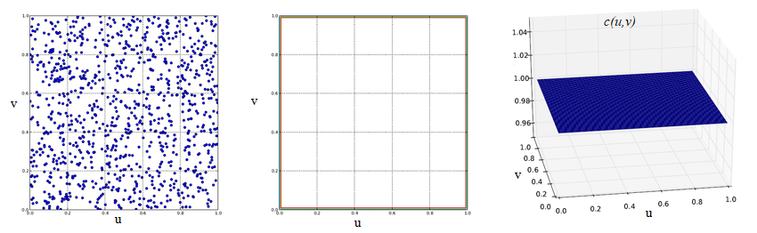
A first example of copulas is the product copula C(u; v) = uv (see, figure 4).
Let X and Y be continuous random variables(r.v.-s) with d.f.-s F(x) = P(X ≤ x) and G(y) = P(Y ≤ y), and joint distribution function (d.f.) H(x, y) = P(X ≤ x, Y ≤ y). The importance of copulas in statistics is described in Sklar’s Theorem (see, [34]).
Theorem 2.3. (Abe Sklar, 1959) Let H be a joint d.f. with margins F and G. Then there exists a copula C such that for all x, y in R,
H (x, y) = C (F (x) , G (y)) . (2.1)
If F and G are continuous, then C is unique; otherwise, C is uniquely determined on Ran (F)× Ran (G) . Conversely, if C is a copula and F and G are d.f.-s, then the function H defined by (2.1) is a joint d.f. with margins F and G.
The representation (2.1) suggests that if the copula C were known, then substituting continu-ous marginal estimators for F and G would yield a plug-in estimate of their associated joint d.f.
Let φ be a continuous, strictly decreasing function from [0, 1] to [0, ∞] such that φ (1) = 0.
Definition 2.4. Copulas of the form
[−1]
C (u, v) = φ (φ (u) + φ (v)) , (2.2)
are called Archimedean copulas, where the function φ is called a generator of the copula φ (1) =
[−1] [−1] −1
0, φ is the pseudo-inverse function of φ. If φ (0) = ∞, then φ = φ .
[−1]
Note that φ is continuous and non-increasing on [0, ∞], and strictly decreasing on [0, φ (0)]. For example, φ (t) = −lnt generator of Gumbel-Hougaard copula.
3. Description of the censoring model with covariates
The problem of estimating multivariate distributions based on censored data began in the early 1980s. For example, the scientific research works of the following scientists can be cited: Gre-gory Campbell (1981), Gregory Campbell & Antonia Földes (1982), James A. Hanley & Milton N. Parnes (1983), Lajos Horváth (1983), Wei-Yann Tsai, Sue Leurgans & John Crowley (1986), Murray D. Burke (1988), Dorota M. Dabrowska (1988, 1989), Richard D. Gill (1992), Abdu-rakhim Abdushukurov (2004), Abdurakhim Abdushukurov & Rustamjon Muradov (2011, 2013, 2022-2024) and others (see, [5]-[7], [18]-[28], [31], [32]). In particular, if the distribution is two-dimensional, the time until the death of people (twins or couples), the failure times of the components of a physical system can be given as random censored variables.
At present time, there are several approaches to estimating of reliability functions of vectors of lifetimes. Moreover, the random variables (r.v.-s) of interest lifetimes and censoring r.v.-s can be also influenced by other variable, often called prognostic factor or covariate. In medicine, dose a drug and in engineering some environmental conditions temperature, pressure and others are influenced to the observed variables (see, [10], [15], [17]).
Let’s consider the case when the support of covariate C is the interval [0, 1] and we consider our results on fixed design points 0 ≤ x1 ≤ x2 ≤ · · · ≤ xn ≤ 1. Thus, on a probability space (Ω, A, P) . Let’s consider two sequences X = {(X1i, X2i) , i ≥ 1} and Y = {(Y1i, Y2i) , i ≥ 1} of conditionally independent random vectors with conditional reliability functions Fx (t, s) = P (X11 > t, X21 > s/C = x) and Gx (t, s) = P (Y11 > t, Y21 > s/C = x) at given covariate ¯ +2 C = x, where x ∈ [0, 1] and (t, s) ∈ R = [0, ∞) × [0, ∞). Here sequences X and Y can be dependent. Introduce a marginal conditional reliability functions
R1x (t) = P (X11 > t/C = x) , R2x (s) = P (X21 > s/C = x) ,
R1x (t) = P (Y11 > t/C = x) , R2x (s) = P (Y21 > s/C = x) , (3.1)
which supposed to be continuous, x ∈ [0, 1] , t, s ≥ 0. Suppose that vector X is censored from the right by vector Y and observed data is consist on V = {(Zi, δi, Ci) , i = 1, . . . , n} , where Zi = (Z1i, Z2i) , Zki = min (Xki, Yki) , δi = (δ1i, δ2i) , δki = I (Zki = Xki) , k = 1, 2 ; i = 1, n. Here I (A) is stands for an indicator of event A. Introduce jointly conditional reliability function of the vector (X11, X21,Y11, Y21) given C = x :
Kx (t, s, z, v) = P (X11 > t, X21 > s, Y11 > z, Y21 > v/C = x) , (t, s, z, v) ∈ R .
Then we obtain representations at x ∈ [0, 1] :
Fx (t, s) = Kx (t, s, 0, 0) , Gx (t, s) = Kx (0, 0, t, s) , (t, s) ∈ R , (3.2)
Hx (t, s) = P (Z11 > t, Z21 > s/C = x) = P (X11 > t, Y11 > t, X21 > s, Y21 > s/C = x) =
= Kx (t, s, t, s) , (t, s) ∈ R . (3.3)
Then according to the Theorem of Sklar (see, [2],[34]), there exist on [0, 1] conditional copula survival function Cx (u) , u = (u1, u2, u3, u4) ∈ [0, 1] such that we have following representation of reliability function (3.2) for all (t, s, z, v) ∈ R as
X X Y Y
Kx (t, s, z, v) = Cx R1x (t) , R2x (s) , R1x (z) , R2x (v) . (3.4)
Assume that at the fixed design value x ∈ [0, 1] , Cx is Archimedean copula, i.e.
[−1] 4
Cx (u1, u2, u3, u4) = φ [φx (u1) + φx (u2) + φx (u3) + φx (u4)] , u ¯ = (u1, u2, u3, u4) ∈ [0, 1] , (3.5) where, for each x, φx : [0, 1] → [0, ∞] is a known continuous, convex, strictly decreasing
[−1]
function with φx (1) = 0, φx is a pseudo-inverse of φx (see, [2], [13]) and given by
[−1] φx (s), 0 ≤ s ≤ φx(0), φx (s) = 0, φx(0) ≤ s ≤ ∞.
[−1] −1
We assume that copula generator function φx is strict, i.e. φx (0) = ∞ and hence φx = φx . Thus from formulas (3.2)-(3.5) one can get for a fixed x ∈ [0, 1]
−1 X X +2
Fx (t, s) = φx φx R (t) + φx R (s) , (t, s) ∈ R ,
1x 2x
−1 Y Y +2
Gx (t, s) = φx φx R (t) + φx R (s) , (t, s) ∈ R , (3.6)
1x 2x
and
−1 X X Y Y +2
Hx (t, s) = φx φx R (t) + φx R (s) + φx R (t) + φx R (s) , (t, s) ∈ R ,
1x 2x 1x 2x
Since
R1x (t) = P (Z11 > t/C = x) = Hx (t; 0) = P (X11 > t, Y11 > t/C = x) , t ≥ 0,
and
R2x (s) = P (Z21 > s/C = x) = Hx (0, s) = P (Y11 > s, Y21 > s/C = x) , s ≥ 0,
then from last formula in (3.2) we obtain
Z −1 X Y
R (t) = φx φx R (t) + φx R (t) , t ≥ 0,
1x 1x 1x Z −1 X Y
R2x (s) = φx φx R2x (s) + φx R2x (s) , s ≥ 0. (3.7) Now from (3.7) it follows that for fixed x ∈ [0, 1]
φx (Hx (t, s)) = φx (Fx (t, s)) + φx (Gx (t, s)) , (t, s) ∈ R .
Note that functionals (3.7) admits to estimation of one dimensional reliability functions R and R correspondingly by subsamples
V = (Z1i, δ1i, Ci) , i = 1, n and V = (Z2i, δ2i, Ci) , i = 1, n
(n) (n) (n) (n)
with V + V = V and then by V estimation of joint reliability function Fx (t, s) using first formula in (3.2). Let H (t) = P (Zki ≤ t, δki = 1/Ci = x) are subdistribution functions and Λkx(t) is crude hazard functions of r.v. Xki, k = 1, 2 subjecting to censoring by Yki for given Ci = x. Then (see, [1]) we have
P (Xki ∈ dt, Xki ≤ Yki/Ci = x) H (dt) Λkx (dt) = = , k = 1, 2. (3.8) P (Xki ≥ t, Yki ≥ t/Ci = x) R (t−)
From (3.4) one can obtain following expressions of reliability functions R :
Zt
X −1 Z Z
Rkx (t) = φ − R (u−) φ R (u) dΛkx (u) =
x kx x kx
Zt
−1 Z (1)
= φx − φx(Rkx (u))dH (u) , t ≥ 0, k = 1, 2, (3.9)
(see, for example, [17]). In order to constructing the estimator of S according to representa-
Z (1)
tion (3.9), we introduce some smoothed estimators of R and H . Similarly to Breakers and
kx kx
Veraverbeke (2005), we will also use the Gasser-Müller weights
xi
1 1 x − u wni(x, hn) = π du, i = 1, ..., n, qn (x, hn) hn hn
xi−1
with
xn
1 x − u qn (x, hn) = π du, hn hn
where x0 = 0, π is a known probability density function (kernel) and {hn, n ≥ 1} is a sequence of positive constants, tending to zero as n → ∞, called bandwidth sequence. Let’s introduce the
Z (1)
weighted estimators of R and H respectively for k = 1, 2 as
kx kx
Rkx (t) = wni (x, hn) I (Zki > t) = 1 − Hkxh(t),
Hkxh(t) = wni (x, hn) I (Zki ≤ t, δki = 1) . (3.10)
Rkx (t) = wni (x, hn) I (Zki > t) = 1 − Hkxh(t),
Hkxh(t) = wni (x, hn) I (Zki ≤ t, δki = 1) .
Zt
−1 Z (1)
Rkxh = φx − φx Rkxh (u) dH (u) , t ≥ 0. (3.11)
Remark that in case of no covariate, estimator (3.11) reduces to estimator first obtained by Zeng and Klein (1995)(see, [29]) for one sample case, which in case of the independent copula φ (y) = − log y, reduces to a exponential hazard estimate. Now we propose second estimator from [15], the extended analogue of relative-risk power estimator introduced in [4], [5] under independent censoring case for k = 1, 2 :
ˆ X −1 ˆ Z Rkxh (t) = φx φx Rkxh (t) µkxh (t) , t ≥ 0, (3.12)
where
X Z −1
µ (t) = φ R (t) φ R ˜ (t) ,
kxh x kxh x kxh
Zt
X Z (1)
φx Rkxh(t) = − φx Rkxh (u) dH (u),
Zt Z Z Z 1 (1) φ R ˆ (t) = − n φ R (u) − φ R (u) − dH (u) ,
x kxh x kxh x kxh
Zt ˜ Z Z φx Rkxh(t) = − φx Rkxh (u) dHkxh (u).
Using estimators (3.11) and (3.12) we can propose two corresponding estimators of the first jointly reliability function in (3.6):
−1 X X +2
Fxh (t, s) = φx φx R1xh (t) + φx R2xh (s) , (t, s) ∈ R ,
−1 X X +2
F ˆ (t, s) = φ φ R ˆ (t) + φ R ˆ (s) , (t, s) ∈ R . (3.13)
xh x x 1xh x 2xh
In order to investigate estimators (3.13) we introduce some conditions. For the design point x1, ..., xn denote ∆ = min (x − x ) , ∆ ¯ = max (x − x ) .
n i i−1 n i i−1 1≤i≤n 1≤i≤n
R ∞ R ∞
2 2 v
For the kernel π, let ∥π∥ = π (u) du, mv (π) = u π (u) du, v = 1, 2, ∥π∥ = sup π (u) .
−∞ −∞ u∈R
Moreover, we use next assumptions on design points and on the kernel function:
1 ¯ 1 A1) As n → ∞, xn → 1, ∆n = O , ∆n − ∆n = o .
A2) π is a probability density function with compact support [−M, M] for some M > 0, with m1 (π) = 0 and |π (u) − π (u )| ≤ C (π) |u − u | , where C (π) is some constant. Let Tk = inf t ≥ 0 : S (t) = 0 , k = 1, 2. For our result we need some smoothness conditions on functions Hkx(t) = P(Zki ≤ t/Ci = x) and H (t) , k = 1, 2. We formulate them for a general (sub) distribution functionNx (t), 0 ≤ x ≤ 1, t ≥ 0 and for a fixed T > 0 :
A3) Nx (t) = Nx (t) exist and continuous in (x, t) ∈ [0, 1] × [0, T] .
A4) Nx (t) = N x (t) exist and continuous in (x, t) ∈ [0, 1] × [0, T] .
A5) 2 Nx (t) = Nx (t) exist and continuous in (x, t) ∈ [0, 1] × [0, T] .
∂ ′′
A6) 2 Nx (t) = N x (t) exist and continuous in (x, t) ∈ [0, 1] × [0, T] .
∂ ˙ ′ A7) Nx (t) = Nx (t) exist and continuous in (x, t) ∈ [0, 1] × [0, T] .
∂x∂t
′ 2 ′′
∂φx(u) ∂ φx(u)
A8) = φ (u) and 2 = φ (u) are Lipschitz in the x− direction with a bounded
∂u x ∂u x
3 ′′′
∂ φx(u)
Lipschitz constant and 3 = φ (u) exist and continuous in (x, t) ∈ [0, 1] × [0, T] .
∂u x
4. Asymptotic properties of estimators
Firstly we establish the asymptotic equivalence of two estimators F ˆ (t , t ) and F (t , t )
xh 1 2 xh 1 2
proposed by formulas (3.13). Let’s denote ∇ = [0, T1] × [0, T2] .
Theorem 4.1. Assume (A1), (A2), functions Hkxh (t) and H (t) satisfy (A5)-(A7) in [0, Tk] , k = 1, 2; φx satisfies (A8). Then as n → ∞ and x ∈ [0, 1] :
a.s. 1 sup F ˆ (t , t ) − F (t , t ) = O . (4.1)
xh 1 2 xh 1 2
(t ,t )∈∇ n Thus for all (t1, t2) ∈ ∇ and x ∈ [0, 1]
F ˆ (t , t ) − F (t , t ) = F (t , t ) − F (t , t ) + q (t , t ) ,
xh 1 2 x 1 2 xh 1 2 x 1 2 n 1 2 a.s. 1
where q (t , t ) = F ˆ (t , t )−F (t , t ) and by Theorem 4.1 sup |q (t , t )| = O .
n 1 2 xh 1 2 xh 1 2 n 1 2 n (t1,t2)∈∇
Hence from two estimators in (3.13) it is enough to investigate only estimator Fxh (t1, t2) . The next result is on almost sure representation of estimator by sums of weighted functions with rate.
Theorem 4.2. Assume (A1), (A2), functions Hkxh (t) and H (t) satisfy (A5)-(A7) in [0, Tk] , k =
log n nhn
1, 2; φx satisfies (A8), hn → 0, → 0 and = O (1) . Then as n → ∞,
nhn log n
Fxh (t1, t2) − Fx (t1, t2) = wni (x, hn) ψkxt (Zi, δi) + rn (t1, t2) ,
k=1,2 i=1
where for k = 1, 2
tk
(−1) ′′ (1) ψkx (Zi, δi) = φ R (u) (I (Zki ≤ u) − Hkx(u)) dH (u)−
tk ′ X x kx kx
φx(R (tk))
′ (1)
−φx Rkx (tk) I (Zki ≤ t, δki = 1) − H (tk) −
tk ′′ (1)
− φx Rkx (u) I (Zki ≤ u, δki = 1) − H (u) dHkx(u) ,
rn (t1, t2) = r1n (t1) + r2n (t2) and
a.s. log n sup |rk (tk)| = O .
0≤t≤T nhn
5. Conclusion
Following results are obtained in the article: Investigated the importance of Archimedean copula functions in statistical modeling. Studied the characteristic properties of the copula function and a visualization graph of the limiting property of a two-dimensional copula has been constructed. Sklar’s theorem was applied to statistical estimation of two-dimensional joint distribution and reliability functions. The asymptotically properties of statistical estimates constructed for relia-bility functions in the presence of covariates are investigated.
Acknowledgment
In conclusion, the authors expresses his sincere gratitude to the professor of Moscow State Uni-versity Tashkent Branch, the Department of Applied Mathematics and Informatics, Professor, Abdurakhim Abdushukurov and reviewer for useful advice.
Figures
The PDF also contains 1 image in a format that could not be extracted automatically.
References
- [1] T. R. Fleming, D. R. Harrington, Counting processes and survival analysis. New York: Wiley, 1991.
- [2] R. B. Nelsen, An introduction to copulas. New York: Springer, 2006.
- [3] A. A. Abdushukurov, Estimates of unknown distributions from incomplete observations and their proper-ties. Germany.: LAP, 2011.
- [4] A. A. Abdushukurov, Nonparametric estimation of the distribution function based on relative risk func-tion. Commun. Statist.: Theory & Methods. 27, (1998), 1991–2012.
- [5] A. A. Abdushukurov, On nonparametric estimation of reliability indices by censored samples. Theory. Probab. Appl. 43, (1999), 3–11.
- [6] A. A. Abdushukurov, Nonparametrical estimators of survival function on the plane by censored observa-tions. Uzbek mathematical journal, 2, (2004), 3–11.
- [7] A. A. Abdushukurov, R. S. Muradov, Estimation of two-dimensional survival function by random right censored data. Proceedings of XI th International Conference "Computer Data Analysis & Modeling", (2016), 81–86.
- [8] A. A. Abdushukurov, Estimation of joint survival function from censored observations. Zavod. Lab. Diagn. Mater., 82, (2016), 80–84.
- [9] A. A. Abdushukurov, R. S. Muradov, On the estimates of the distribution function in a random censorship model. Zavod. Lab. Diagn. Mater.. 80, (2014), 62–67.
- [10] A. A. Abdushukurov, R. S. Muradov, On Estimation of Conditional Distribution Function under Depen-dent Random Right Censored Data. Journal of Siberian Federal University. Mathematics & Physics 7, (2014), 409–416.
- [11] A. A. Abdushukurov, R. S. Muradov, Estimation of survival functions from dependent random right cen-sored data. Intern. J. Innovation in Science and Mathematics, 2, (2014), 280–287.
- [12] A. A. Abdushukurov, N. Nurmuhamedova, S. Bozorov, Nonparametric Estimation of Distribution Func-tion Under Right Random Censoring Based on Presmoothed Relative-Risk Function. Lobachevskii Jour-nal of Mathematics, 42(2), (2021), 257–268.
- [13] A. A. Abdushukurov, R. S. Muradov, Some algebraic properties of Archimedean copula functions and their applications in the statistical estimation of the survival function. New Trends in Math. Sci., 4, (2014), 88–98.
- [14] A. A. Abdushukurov, R. S. Muradov, Estimation of bivariate survival function from random censored data with Poisson sample size. Calcutta Statistical Association Bulletin., 72(2), (2020), 111-122.
- [15] A. A. Abdushukurov, Estimation of conditional survival function under dependent right random censored data. Austrian J. of Statist., 49, (2020), 1–8.
- [16] A. A. Abdushukurov, R. S. Muradov, On Estimation of Bivariate Survival Function from Random Cen-sored Data. Journal of Siberian Federal University. Mathematics & Physics., 13(4), (2020), 422–430.
- [17] R. Braekers, N. Veraverbeke, A copula graphic estimator for the conditional survival function under dependent censoring. Canadian J. Statist., 33(3),(2005), 429–447.
- [18] M. D. Burke, Estimation of a bivariate distribution function under random censorship. Biometrika, 75, (1988), 379–382.
- [19] G. Campbell, Nonparametric bivariate estimation with randomly censored data. Biometrika, 68,(1981), 417–422.
- [20] G. Campbell, A. Földes, Lange sample properties of nonparametric bivariate estimators with censored data. Colloquia Mathematica-Societatis János Bolyai, 32, (1982), 103–122.
- [21] D. M. Dabrowska, Kaplan Meier estimate on the plane. Ann. Statist.., 16,(1988), 1475–1489.
- [22] D. M. Dabrowska, Kaplan Meier estimate on the plane: weak convergence, LIL and the bootstrap. J. Multivar. Anal.., 29,(1989), 308–325.
- [23] R. D. Gill, Multivariate Survival Analysis I. Theory Probab. Appl.., 37, (1992), 19–35.
- [24] R. D. Gill, Multivariate Survival Analysis II. Theory Probab. Appl.., 37, (1992), 307–328.
- [25] J. A. Hanley, M. N. Parnes, Nonparametric estimation of a multivariate distribution in the presence of censoring. Biometrika, 68, (1983), 129–139.
- [26] L. Horváth, The rate of strong uniform consistency for the multivariate product-limit estimator. Colloquia Mathematica-Societatis János Bolyai, 13, (1983), 202–209.
- [27] Y. Huang, Two sample multistate accelerated sojourn times model. J.A.S.A.., 95, (2000), 619–627.
- [28] W. Y. Tsai, S. Leurgans, J. Crowley, Nonparametric estimation of a bivariate survival function in the presence of censoring. Ann. Statist., 14, (1986), 1351–1365.
- [29] M. Zeng, J. P. Klein, Estimates of marginal survival for dependent competing risks based on an assumed copula. Biometrika, 82, (1995), 122–128.
- [30] A. A. Abdushukurov, R. S. Muradov, Estimation of conditional jointly survival function under dependent right random censored data. Lobachevskii Journal of Mathematics, 72(4), (2022), 2111-2122.
- [31] A. A. Abdushukurov, N. T. Dushatov, R. S. Muradov, Estimation of Functionals of Multivariate Distri-bution by Censored Observation via Copula Function. Journal of Mathematical Sciences, 267(1), (2022), 108-116.
- [32] A. A. Abdushukurov, N. T. Dushatov, R. S. Muradov, Nonparametric estimators of bivariate distributions from incomplete samples and their applicationsþ Journal of Mathematical Sciences, 267(1), (2022), 16- 22.
- [33] F. Durante, C. Sempi, Principles of copula theory. Taylor & Francis Group, LLC, New York, (2016).
- [34] A. Sklar, Random variables, joint distribution functions and copulas. Kybernetika, Prague, 9, (1973).449- 460. Author information Rustamjon Muradov, Department of Higher Mathematics, Namangan Institute of Engineering and Technology, Namangan, 160115, UZBEKISTAN. E-mail: rustamjonmuradov@gmail.com Abdurakhim Abdushukurov, Department of Applied Mathematics and Informatics, Moscow State University Tashkent Branch, Tashkent 100000, UZBEKISTAN. E-mail: a_abdushukurov@rambler.ru Received: 02.04.2024 Accepted: 25.05.2024 Published: 30.06.2024