
NEW ASPECTS OF CERTAIN SPECIAL FUNCTIONS WITH APPLICATIONS
Abstract
Throughout the history of natural science, special functions (SFs) have been a powerful instrument in the solution of a wide variety of important problems in various fields such as physics, engineering, biology, medicine, economics, and finance. The reduction of any given applied problem to the evaluation of special functions has always been, and still is, looked on as indicating a strong penetration into the essence of the problem. Almost all the familiar special functions have arisen from a wide diversity of applied problems, so the study of their proper-ties and their applications has engaged not only mathematics but also physicists, astronomers, engineers, and other specialists.
Furthermore, fractional calculus of special functions, which perform fractional differentiation or integration of functions, is gaining popularity due to its numerous scientific, technological, and engineering applications. So, the current review article dives into recent mathematical findings on generalizations of special functions and polynomials related to various fractional calculus operators (FCOs). Also emphasized is their importance and extensive utility in dealing with the most well-known topics: integral transformations, initial value problems, and kinetic equations.
More precisely, we discuss analytic properties and numerical exemplifications of extensions Beta and hypergeometric functions associated with fractional calculus operators. Moreover, some developments and applications of orthogonal matrix polynomials, such as the generalized Bessel matrix polynomials and the generalized Jacobi matrix polynomials, have been consid-ered. Furthermore, novel generalizations of fractional kinetic equations involving certain special functions and their solutions using the various integral transforms have been shown. Finally, some important points that can be suitable to be future works are summarized.
Keywords and phrases: Special functions, fractional operators, integral transforms, Frac-tional kinetic equations.
MSC 2020 Classifications: 33C20, 33C20, 26A33, 35R11.
1. Introduction
1.1 What are the special functions?
The concept of special functions (SFs) refers to a class of mathematical functions that appear in a variety of situations, most notably in differential equation, mathematical physics, chemistry, and other fields, see, for instance, Sneddon (1956)[1], Nikiforov and Uvarov (1988)[2], and Bell (2004)[3]. These functions frequently possess unique qualities, behaviors, or forms that make them very valuable in applications. Moreover, the term special functions is applied to functions that are not trivial. In some sense the polynomials are the most special of all to the extent of being boring. The next simplest is the family of exponential functions the usual real exponential, the trigonometric and hyperbolic functions, and the general complex exponential that incorpo-rates all of them and their inverse functions. These may have been supposed to be boring but, as we shall see, they are interesting. They can be taken as solutions of first-order differential equa-tions. The next lot of special functions is the solutions of the linear second-order differential equations of mathematical physics and engineering. These include the Legendre polynomials and functions, the Laguerre, the Hermite, the Chebyshev, the Jacobi,the Gegenbauer, the Bessel and related functions and some others. All of them arise as special cases of the generalized hypergeometric functions U = pFq of p numerator and q denominator parameters (see, Dwork (1990) [4]) that are solutions of the differential equation
Y d d Y d z z + αk U = z z + βk − 1 U, (1.1) dz dz dz
k=1 k=1
where
α1 α2 · · · αp ∞ (α1)m · · · (αp)m z pFq ; z = , (1.2) (β1)m · · · (βq)m m!
β β · · · β m=0
1 2 q
and (a)m is the usual Pochhammer symbol (or the rising factorial). For p = 2 and q = 1, we get the Gauss hypergeometric function 2F1.
The other functions are those that arose in the theory of numbers. It is of interest to follow them in more detail. The first of them, the Gamma function (Euler integral of the second kind), a generalization of the factorial function defined for integers to the real domain and thence to the complex domain (see, Davis (1959) [5]):
−y κ−1
Γ(κ) := e y dy, Re(κ) > 0. (1.3)
The function Γ is closely related to the Beta function (Euler integral of the first kind)
κ1−1 κ2−1
B(κ1, κ2) = y (1 − y) dy
Γ(κ1)Γ(κ2) = Re(κ1, κ2) > 0.
Γ(κ1 + κ2)
By using the Gamma function (1.3). Swedish Mathematician Gosta Mittag-Leffler (1903) [6] introduced the following Mittag-Leffler function of one parameter
Eα(y) = , Re(α) > 0. (1.5) Γ(rα + 1)
This function is the direct generalization of the exponential function and is known as the queen of the functions of fractional calculus. For other generalizations, properties, and applications of the Mittag-Leffler functions, the reader might consult the work by Haubold et al. (2001)[7].
Further, SFs are often highly studied, and their properties such as differential (or differ-ence ) equations, asymptotic behavior, recurrence relations, integral formulas, orthogonality, Rodrigues’ formulas, and generating functions, are extensively documented. These attributes render them effective tools for swiftly addressing intricate issues.
On top of that, recently special matrix functions (SMFs) appear in connection with statistics, Lie group theory, and theoretical physics. Many authors have dealt with orthogonal matrix poly-nomials and their applications, For examples, Hermite, Laguerre, Chebyshev, Jacobi, Gegen-bauer, Bessel and Legendre matrix polynomials were introduced and established, see, tutorial survey by Abdalla (2020) [8].
Next, further details will be provided about the importance of relationships between SFs and both fractional calculus operators (FCOs) and integral transforms (ITs).
1.2 Fractional calculus operators
The notion “Fractional Calculus” (FC) or “Fractional Analysis” is used for the extension of the Calculus (Analysis), when the order of integration and differentiation can be an arbitrary number (fractional, irrational, complex), that is, not obligatory integer. The FC is nowadays one of the most rapidly growing subjects of mathematical analysis in spite of the fact that it is nearly 300 years old. Where the giants of mathematics, W. Leibniz (1697), L. Euler (1730), thought about the possibility to perform differentiation of non-integer order.
The real birth and far-reaching development of the FC is due to numerous attempts of math-ematicians during the nineteenth century to beginning of twentieth century. It is practically impossible to name all important contributions made in construction of early stages of building of the FC. For example, see the survey by Machado and Kiryakova (2010)[9, 10], Machado et al. (2010)[11].
In the same vein, fractional calculus operators (FCOs), which handle non-integer (fractional) ordering on functions as a type integral transform convolutions. It is an extension of classical operators, which originated and developed with the pioneering contributions of Lacroix (1819), Liouville (1832), Letnikov (1868), Riemann (1876), Hadamard (1892), Weyl (1919), Caputo (1967) and numerous others [12]. In the literature, FCOs are defined in a wide variety of ways. Two widely used operators are the Riemann-Liouville and Caputo fractional operators [13]. Nev-ertheless, among the monographs developing the theory of FCOs involving various special func-tions and presenting some applications, we have to point out works by, Oldham and Spanier (1974) [14], Lovoie (1976)[15] Kilbas (2005) [16], Kiryakova (2008)-(2020)[17, 18], Srivastava (2015)[19], Kochubei (2019)[20], Sandev (2022)[21], and Singh (2023)[22].
Let us now begin with some various representations for FCOs.
The Riemann-Liouville-Caputo fractional operators
The Riemann-Liouville fractional integral operator (RLFIO) of order ν, introduced by Bernhard Riemann and Joseph Liouville, is defined as
−ν ν 1 ν−1 0Dw f(w) := (I f)(w) := (w − u) f(u)du, Re(ν) > 0, (1.6) Γ(ν) 0
where Γ denots the Gamma function defined in (1.3), and the Riemann-Liouville fractional dif-ferential operator (RLFDO) of order µ, defined as
µ n n−µ
Dwf(w) := D I f(w) , n − 1 < Re(µ) < n. (1.7)
In 1967, Italian Caputo defined the Caputo fractional derivative operator (CFDO) as
µ 1 n−µ−1 d Dwf(w) := (w − u) f(u)dt, (1.8) Γ(n − µ) 0 du
where n − 1 < Re(µ) < n.
Recently, many generalizations of RLFOs and CFDOs have been considered, such as the Hil-fer, Hadamard, Katugampola, Hilfer-Caputo, and Hadamard-Caputo fractional operators, extend of (1.6), (1.7) and (1.8) by introducing additional parameters or kernel functions. In particular, Mubeen and Habibullah (2012) [23] defined the k−RLFIO by
υ −1
I f(τ) (x) = f(τ)(x − τ) k dτ; υ, k > 0. (1.9) kΓ (υ) 0
Due to this, the k− RLFIO of order υ introduced by Rahman et al. (2020) [?] as
υ (1−υ) d Dk f(η) = D I f(η) ; 0 < υ ≤ 1, D = . (1.10) dη
where Γ (y) is the k−Gamma function k y−1 − −
Γ (y) = u e k du, y ∈ C \ kZ . (1.11)
These formulas have been applied in many recent works (see, e.g., [24, 25, 26])
The Hadamard fractional operators
Definition 1.1. [27] Let 0 ≤ a ≤ b ≤ ∞, be finite or infinite interval of the half-axis R . The Hadamard fractional integral operators of order α ∈ C are defined by
1 x α−1 dt (HIa+φ) (x) = log φ(t) , a < x < b, Γ(α) a t t Z (1.12)
b α−1
α 1 t dt HIb−φ (x) = log φ(t) , a < x < b.
Γ(α) x x t The left-sided and right-sided Hadamard fractional derivative operators of order α ∈ C, n ∈ N with Re(α) ≥ 0 on (a, b) and a < x < b are defined by
α n n−α
(HDa+φ) (x) = δ HIa+ φ (x) n Z x d 1 x n−α−1 φ(t)dt = x log , dx Γ(n − α) a t t
α n n−α
HDb−φ (x) = (−δ) HI φ (x) n Z b n−α−1 d 1 t φ(t)dt = −x log .
dx Γ(n − α) x x t
If Re(α) > 0, Re(β) > 0 and 0 < a < b < ∞, then we have
t Γ(β) x β+α−1 HIa+ log (x) = log , a Γ(β + α) a
and (1.14)
t Γ(β) x β−α−1 HDa+ log (x) = log .
a Γ(β − α) a
The Marichev-Saigo-Maeda fractional operators
In 1974, Marichev [28] introduced fractional integral operators as Mellin type convolution op-erator with the Appell function F3 in their kernel. In the middle of the 1990s, these fractional integral operators were rediscovered and studied by Saigo (1978-1980) [29, 30], extended and investegated later after that by Saigo and Maeda (1996) [31] and by Saigo and Saxena (2001) [32] as generalizations of the celebrated Saigo fractional integral operators.
The generalized fractional calculus operators (the Marichev-Saigo-Maeda operators) involv-ing the Appell’s function or Horn’s F3 function in the kernel are defined as follows:
Definition 1.2. Let σ, σ , v, ν , η ∈ C and x > 0, then for Re(η) > 0
σ,σ ,v,v ,η
I f (x) Z x (1.15) x ′ t x
η−1 −σ ′ ′
= (x − t) t F3 σ, σ , v, v ; η; 1 − , 1 − f(t)dt, Γ(η) 0 x t
σ,σ ,v,v ,η
Ix,∞ f (x) ′ Z (1.16)
−σ ∞
x η−1 −σ ′ ′ x t = (t − x) t F3 σ, σ , v, v ; η; 1 − , 1 − f(t)dt, Γ(η) x t x provided that the function f(t) is so constrained such that the integrals in Equations (1.15) and (1.16) exist.
In Equations (1.15) and (1.16), F3 denotes the Appell’s hypergeometric function [33] in two variables defined as:
F3 (σ, σ , v, v ; η; x, y)
∞ ′ ′ m n
X (σ) (σ ) (ν) (v ) x x (1.17)
m n m n
= , (max{|x|, |y|} < 1).
(η)m+n m! n!
m,n=0
Then the above fractional integral operators in Equations (1.15) and (1.16), can be written as follows:
′ ′ d ′ ′
σ,σ ,ν,v ,η σ,σ ,ν+k,v ,η+k
I f (x) = I f (x)
0,x 0,x
dx (1.18) (Re(η) < 0; k = [− Re(η) + 1]),
′ ′ d ′ ′
σ,σ ,v,v ,η σ,σ ,v,ν +k,η+k
Ix,∞ f (x) = − Ix,∞ f (x) dx (1.19) (Re(η) < 0; k = [− Re(η) + 1]).
Remark 1.3. It is worthy to note that the Appell function defined in Equation (1.17) reduces to the Gauss hypergeometric function 2F1 as given in the following relations:
F3(σ, η − σ, v, η − v; η; x, y) = 2F1(σ, v; η; x + y − xy),
also we have
F3 (σ, 0, v, v , η; x, y) = 2F1(σ, v; η; x),
′ ′ ′ ′
F3 (0, σ , v, v , η; x, y) = 2F1 (σ , v ; η; y) .
The corresponding Marichev-Saigo-Maeda fractional differential operators are given as fol-lows:
Definition 1.4. Let σ, σ , v, v , η ∈ C and x > 0, Then
′ ′ ′ ′
σ,σ ,v,v ,η −σ ,−σ,−v ,−v,−η
D f (x) = I f (x)
0,x 0,x
d ′ ′
−σ ,−σ,−v +k,−v,−η+k
= I f (x), (Re(η) > 0; k = [Re(η)] + 1) dx k Z (1.20) 1 d ′
σ k−η−1 σ
= (x) (x − t) t Γ(k − η) dx 0
′ ′ t x × F3 −σ , −σ, k − v , −v; k − η; 1 − , 1 − f(t)dt, ′ ′ ′ ′
σ,σ ,v,v ,η −σ ,−σ,−v ,−v,−η
Dx,∞ f (x) = Ix,∞ f (x)
d ′ ′
−σ ,−σ,−v ,−v+k,−η+k
= − Ix,∞ f (x), (Re(η) > 0; k = [Re(η)] + 1) dx k Z (1.21) 1 d ′
σ k−η−1 σ
= − (x) (t − x) t Γ(k − η) dx x
′ ′ x t × F3 −σ , −σ, −v , k − v; k − η; 1 − , 1 − f(t)dt.
In view of the above reduction formula as given in Equation (2.7), the generalized fractional calculus operators reduce to the Saigo operators [?] defined as follows:
Definition 1.5. Let x > 0, σ, ν, η ∈ C and Re(σ) > 0, then
−σ−v
σ,v,η x σ−1 t I f (x) = (x − t) 2F1 σ + v, −η; σ; 1 − f(t)dt, Γ(σ) 0 x
σ,v,η 1 σ−1 −σ−v x Ix,∞ f (x) = (t − x) t 2F1 σ + v, −η; σ; 1 − f(t)dt.
Γ(σ) x t
The Saigo fractional integral operators, given in Equations (2.11) and (2.12) can also be written as:
Let x > 0, σ, v, η ∈ C, then
σ,v,η d σ+k,v−k,η−k I f (x) = I f (x)
0,x 0,x
dx (Re(σ) < 0; k = [Re(−σ)] + 1),
σ,v,η d σ−k,ν−k,η Ix,∞ f (x) = − Ix,∞ f (x) dx (Re(σ) < 0; k = [Re(−σ)] + 1).
The corresponding Saigo fractional differential operators are defined as:
Definition 1.6. Let σ, v, η ∈ C and x > 0. Then
σ,v,η −σ,−v,σ+η d −σ+k,−v−k,σ+η−k D f (x) = I f (x) = I f (x)
0,x 0,x 0,x
dx (Re(σ) > 0; k = [Re(σ)] + 1),
σ,ν,η −σ,−ν,σ+η d −σ+k,−ν−k,σ+η Dx,∞ f (x) = Ix,∞ f (x) = − Ix,∞ f (x) dx (Re(σ) > 0; k = [Re(σ)] + 1),
where [x] denotes the integer part of x.
If we take v = 0 in Equations (2.11), (2.12), (2.15) and (2.16), we get the socalled Erdélyi-Kober fractional integral and derivative operators defined as follows[34]:
Definition 1.7. Let x > 0, σ, η ∈ C with Re(σ) > 0, then
−σ−η
σ,η x σ−1 η I f (x) = (x − t) t f(t)dt, Γ(σ) 0
σ,η x σ−1 −σ−η Ix,∞ f (x) = (t − x) t f(t)dt.
Γ(σ) x provided that integrals in Equations (2.17) and (2.18) converge.
The corresponding derivative operators are defined as:
Definition 1.8. Let x > 0, σ, η ∈ C with Re(σ) > 0, then
k Z x σ,η −η d 1 σ+η k−σ−1 D f (x) =x t (x − t) f(t)dt dx Γ(k − σ) 0
d −σ+k,−σ,σ+η−k = I f (x), (k = [Re(σ)] + 1), dx
k Z ∞ σ,η η+σ d 1 −η k−σ−1 Dx,∞ f (x) =x t (t − x) f(t)dt dx Γ(k − σ) x
k d −σ+k,−σ,σ+η = (−1) Ix,∞ f (x), (k = [Re(σ)] + 1).
dx
When v = −σ, the operators in Equations (2.11), (2.12), (2.15) and (2.16) give the Riemann-Liouville and the Weyl fractional integral operators are defined as follows:
Definition 1.9. Let x > 0, σ ∈ C with Re(σ) > 0, then
σ 1 σ−1 I0,x f (x) = (x − t) f(t)dt, Γ(σ) 0
σ 1 σ−1 Ix,∞ f (x) = (t − x) f(t)dt.
Γ(σ) x provided that both integrals converge.
The corresponding derivative operators are defined as follows:
Definition 1.10. Let x > 0, σ ∈ C with Re(σ) > 0, then
k Z x σ d 1 k−σ−1 D0,x f (x) = (x − t) f(t)dt dx Γ(k − σ) 0
d k−σ = I f (x), (k = [Re(σ)] + 1), dx k Z ∞ σ k d 1 k−σ−1 Dx,∞ f (x) = (−1) (t − x) f(t)dt dx Γ(k − σ) x
k d k−σ = (−1) Ix,∞ f (x), (k = [Re(σ)] + 1).
dx
For more detail about such operators along with their properties and applications, one may refer [35, 36, 37].
Power functions formulas of the above discussed fractional operators required for our present study are given in the following lemmas (see [30, 31, 32]):
Lemma 1.11. Let σ, σ , v, ν , η and ρ ∈ C, x > 0 be such that Re(η) > 0, then the following formulas hold true:
σ,σ ,v,v ,η ρ−1
I t (x)
′ ′ ′
Γ(ρ)Γ (ρ + η − σ − σ − v) Γ (ρ + v − σ ) ′
ρ+η−σ−σ −1 ′ ′ ′
Γ (ρ + v ) Γ (ρ + η − σ − σ ) Γ (ρ + η − σ − v)
′ ′ ′
(Re(ρ) > max {0, Re (σ + σ + v − η) Re (σ − v )}) ,
σ,σ ,ν,v ,η ρ−1
Ix,∞ t (x)
Γ(1 − ρ − v)Γ (1 − ρ − η + σ + σ ) Γ (1 − ρ − η + σ + v ) ′
ρ+η−σ−σ −1
Γ(1 − ρ)Γ (1 − ρ − η + σ + σ + ν ) Γ(1 − ρ + σ − v) (Re(ρ) < 1 + min {Re(−v), Re (σ + σ − η) , Re (σ + v − η)}) .
Lemma 1.12. Let σ, σ , v, ν , η and ρ ∈ C, x > 0 be such that Re(η) > 0, then the following formulas hold true:
σ,σ ,v,v ,η ρ−1
D t (x)
Γ(ρ)Γ (ρ − η + σ + σ + v ) Γ(ρ − v + σ) ′
ρ−η+σ+σ −1
Γ(ρ − v)Γ (ρ − η + σ + σ ) Γ (ρ − η + σ + v ) (Re(ρ) > max {0, Re (η − σ − σ − v ) , Re(ν − σ)}) ,
σ,σ ,v,v ,η ρ−1
Dx,∞ t (x)
′ ′ ′
Γ (1 − ρ + v ) Γ (1 − ρ + η − σ − σ ) Γ (1 − ρ + η − σ − v) ′
ρ−η+σ+σ −1 ′ ′ ′
Γ(1 − ρ)Γ (1 − ρ + η − σ − σ − v) Γ (1 − ρ − σ + v )
′ ′ ′
(Re(ρ) < 1 + min {Re (v ) , Re (η − σ − σ ) , Re (η − σ − v)}) .
2. Integral Transforms
The integral transform (IT) is a mathematical method for translating a differential equation into an algebraic equation. By using this method, a challenging mathematical issue can be reduced to a more manageable one. By integrating the result of a function and another function, known as the kernel of the integral transform, the integral transform mathematical operator can create a result function. The integral transform can be expressed generally as follows:
F(κ) = T(f(y)) = f(y)K(y, κ)dy,
where, F(κ) represents the function produced by the integral transform and K(y, κ) a kernel function. The inverse integral transform is given by
f(y) = T(f(κ))K (κ, y)dκ,
where K (κ, y) is the kernel of the inverse integral transform.
We will now provide a discussion of a number of significant integral transforms.
2.1 Fourier transform
The Fourier transform, the Fourier cosine transform, and the Fourier sine transform can be ef-fectively used for solving differential and integral equations. These transforms are also use-ful in evaluating integrals involving special functions. The reader may refer, for example to, [35, 36, 37, 38].
If f is an absolutely integrable function, the Fourier transforms are defined by [35, 36]
−2πkit
F{f(t)} = F(k) = f(t)e dt, k ∈ R,
and Z
−1 2πikt
F {F(k)} = f(t) = F(k)e dk.
Further, the fractional Fourier transform (FFT) of order β; 0 < β ≤ 1, is defined as
iω β ξ
φβ(ω) = Fβ[φ](ω) = e φ(ξ)dξ, i = −1. (2.1)
2.2 Laplace transform
The Laplace transform of f(t) is formally defined by [35, 36]
¯ −st L{f(t)} = f(s) = e f(t)dt, Re s > 0, (2.2)
The inverse Laplace transform is Z c+i∞ −1 1 st L {f¯(s)} = f(t) = e f¯(s)ds, c > 0. (2.3) 2πi c−i∞
The Laplace transform is highly efficient for solving some class of ordinary and partial differ-ential equations. A variety of extended Laplace-type transforms are introduced for example in [36, 37, 38, 39, 40].
2.3 Pathway-type transform
The pathway-type transform (Pς−transform) is given in [41, 42] in the form
P [f(w), φ] = F(φ) = [1 + (ς − 1)φ] ς−1 f(w)dw ς > 1, (2.4)
with
−ϕw
lim [1 + (ς − 1)φ] ς−1 = e , (2.5)
ς→1+ lim Pς[f(w), φ] = L[f(w), φ], (2.6)
ς→1+
where (L[., .]) is the Laplace transform (2.2).
Some basic results of the Pς− transform are given in [41] as follows
ς − 1 Pς[1, φ] = , (2.7) ln[1 + (ς − 1)φ]
n oυ+1 υ ς − 1 Pς[w , φ] = Γ(υ + 1), υ ∈ C, (2.8) ln[1 + (ς − 1)φ]
h iα −α ς − 1 Pς[ 0Dw f(w), φ] = Pς[f(w), φ], Re(α) > 0, ς > 1, (2.9) ln[1 + (ς − 1)φ]
where 0Dw f(w) is given in (1.6).
More information about the Pς−transform and its applications may be found in [41, 42].
2.4 Hankel transform
The Hankel transform (also designated as Fourier-Bessel transform) is a fundamental tool in many areas of mathematical statistics, physics, engineering, probability theory, analytic number theory, data analysis, etc (see, for instance, [41, 42, 43, 44, 45, 46]). The integral
Hν{f(t); q} = q Jν(qt) f(t) dt, q > 0, R(ν) > , (2.10)
th
defines the Hankel transform involving the ν -order Bessel function of first kind Jν(η) [45] as a kernel. Its inverse transform is
−1 ˜ ˜ f(t) = Hν {f(q)}(t) = qJν(tq)f(q)dq, t > 0. (2.11)
2.5 Mellin transform
The Mellin integral transform is similar with the Laplace transform and Fourier transform and is widely applied in computer science and number theory due to its invariant properties [35, 36]. The Mellin transform of a suitable integrable function f(t) is defined by n o Z ∞ ˜ p−1 f(p) = M f(t) (p) = t f(t) dt, p ∈ C, (2.12)
provided that the improper integral in (2.12) exists. The inverse Mellin transform is n o Z c+i∞ −1 1 −p f(t) = M f˜(p) (t) = t f˜(p) dp, (2.13) 2πi c−i∞
where c ∈ \{p} is a constant.
Further, there are two convolution Type theorems for the Mellin transform. If M{f(t)} = f˜(p) and M{g(t)} = g ˜(p), then
t dξ M[f(t) ∗ g(t)] = M f(ξ)g = f˜(p)g ˜(p), 0 ξ ξ Z (2.14) M[f(t) ◦ g(t)] = M f(tξ)g(ξ)dξ = f˜(p)g ˜(1 − p).
2.6 Beta transform
The Beta transform of f(z) is defined as [48, 49]:
a−1 b−1
B{f(z) : a, b} = z (1 − z) f(z)dz. (2.15)
The matrix version of the Beta transform of f(z) is defined as
P −I Q−I
B{f(z) : P, Q} = z (1 − z) f(z)dz, (2.16)
where P and Q are positive stable matrices in the complex matrix space of common order n; C .
For f(z) = 1, we get the Beta matrix function given by Jodar and Cortés (1998) [50] as
P −I Q−I
B (P, Q) = t (1 − t) dt. (2.17)
2.7 Whittaker transform
The Whittaker transform is defined in [51] as
W(z) = (2zt) 4 W (2zt) f(t) dt, (2.18)
whereWλ,µ(t) is the Whittaker function. For λ = and µ = ± the Whittaker transform goes over into the Laplace transform.
3. Fractional Kinetic Equations
The kinetic (reaction-type) equations have prime importance as mathematical tools widely used in describing several astrophysical and physical phenomena. The production and destruction of nuclei in the chemical (thermonuclear) reactions can be described by the reaction-type (kinetic) equations. Reactions characterized by a time dependent quantity N = N(t) can be formally represented by the following Cauchy problem (See, Haubold and Mathai [52])
dN = −δ(N) + p(N), N(0) = N0, (3.1) dt where δ and p are the destruction rate and the production rate of N, respectively, and N0 is the initial data. Haubold and Mathai [52] studied the following special case of the Cauchy problem,
dN + = −ϑN, ϑ ∈ , N(0) = N0. (3.2) dt Equation (3.2) is known as the standard kinetic equation. An alternative form of equation (3.2) can be obtained as
−1 +
N(t) − N0 = −ϑ 0Dt N(t), ϑ, t ∈ R , (3.3)
where 0Dt is the standard integral operator. Haubold and Mathai [52] have introduced a frac-tional generalization of the standard kinetic equation (3.3) as
ν −ν +
N(t) − N0 = −ϑ 0Dt N(t), ϑ, t ∈ R , (3.4)
where 0Dt is defined in (1.6). The solution of the fractional kinetic equation (3.4) takes the form X (−1)
νn
N(t) = N0 (ϑt) . (3.5) Γ(νn + 1)
Further extensions and generalizations of kinetic fractional equations involving many fractional operators have grown interest in applied science not only in mathematics but also in dynamical systems, physical phenomena, engineering and control systems (see, [53, 54, 55]).
4. Related Works
Several research have been conducted to study generalizations of the SFs. This section reviews some works related to the generalized SFs associated with FCOs and ITs.
4.1 Fractional operators for the Wright hypergeometric matrix function
The generalized (Wright) hypergeometric function were first studied by Virchenko et al.(2001)[56] as follows
Γ(c) X (a) Γ(b + τ n) z
(τ) n
2R (a, b; c; z) = , τ > 0, |z| < 1. (4.1) Γ(b) Γ(c + τ n) n!
The matrix version of (4.1) was introduced by Bakhet et al. (2019) [57] as follows,
Definition 4.1. Let A, B and C be positive stable matrices in C such that the matrix C + nI is invertible for every integer n ≥ 0. Then, the Wright hypergeometric matrix function (WHMF) is defined in the form:
(τ) −1
2R (A, B; C; z) :=Γ (B)Γ(C) X z (4.2) × (A)nΓ (C + τ nI)Γ(B + τ nI) ,
where τ ∈ R+ = (0, ∞) for all integer n ≥ 0, and
A(A + I)...(A + (n − 1)I) = Γ (A)Γ(A + nI), n ≥ 1, (A)n = (4.3) I, n = 0,
is the Pochhammer symbol of a matrix A, where
−w A−I A−I
Γ(A) = e w dw, w = exp((A − I) ln w), (4.4)
is the Gamma matrix function (see [57]). For τ = 1, (4.2) reduces to the Gauss hypergeometric matrix function which is defined by Jódar and Cortés (1998) [50].
In this section, we investigate new properties of the WHMF in (4.2). Further, we introduce the Wright type hypergeometric matrix functions by using the FCOs in (1.6) and (1.7), as follows,
R(w; A, B; ν; λ) = 2F1(A, B; (ν + 1)I; λw) Γ(ν + 1)
w, ν, λ ∈ C and A, B ∈ C ,
R(w; A, B; −µ; λ) = 2F1(A, B; (1 − µ)I; λw) Γ(1 − µ)
w, µ, λ ∈ C and A, B ∈ C .
• Main Results
Theorem 4.2. [58]. Let A, B and C be positive stable matrices in C . Then for τ > 0, m > 0, the following integrals hold true:
∞ m ∞
−u X
C−(τ+1)I
exp u (A)n Γ(B + τ nI)Γ(C)
−1 −1 −1 C − (τ + n)I n (4.7) × Γ (B)Γ (C + τ nI)Γ u du
C−τ I
z (τ) = 2R (A, B; C; z), |z| < 1.
Z 1 (τ) (τ) 2R (A, B; (m + 1)I; 1)
m τ 1
z 2R (A, B; mI; z )dz =
2R (A, B; (m + 2)I; 1) − , |z | < 1.
m(m + 1)
Theorem 4.3. [58]. Let A and B be positive stable matrices in C such that B + nI is invertible for all integer n ≥ 0 and |z| < 1, then
(τ) (τ)
(s + 1) 2R (A, B; (s + 1)I; z) − 2R (A, B; (s + 2)I; z)
τ 2 d (τ) τ = } z 2R (A, B; (s + 3)I; z) + z {τ + 2(s + 1) 2 1 (4.9) (s + 2) dz (s + 2)
d (τ) (τ) × 2R (A, B; (s + 3)I; z) + s 2R (A, B; (s + 3)I; z), Re(s) > 0.
dz
Theorem 4.4. [58]. Let A and B be positive stable matrices in C with B + nI is invertible for all integer n ≥ 0 and λ, µ ∈ C such that |λw| < 1, Re(µ) < 1. Then
I R(w; A, B; ν; λ) = R(w; A, B; ν + γ; λ), (4.10)
D R(w; A, B; ν; λ) = R(w; A, B; ν − γ; λ), (4.11)
I R(w; A, B; −µ; λ) = R(w; A, B; γ − µ; λ), (4.12)
D Rw(A, B; ν; λ) = R(w; A, B; −(γ + µ); λ). (4.13)
Theorem 4.5. [58]. Let C be a positive stable matrix in C , The Laplace transform of R(w; −nI, C + (n − 1)I; ν; λ) and R(w; −nI, C + (n − 1)I; −µ; λ); n ∈ N are given as
L R(w; −nI, C + (n − 1)I; ν; λ) = Yn(C; λ, −s), (4.14)
L R(w; −nI, C + (n − 1)I; −µ; λ) = Yn(C; λ, −s), (4.15)
where Yn(C; λ, −s) is the generalized Bessel matrix polynomial [58].
4.2 Results on the generalized hypergeometric matrix functions
The generalized Gauss and Confluent hypergeometric matrix functions are presented by Abdall et al. (2021) [60] as follows.
∗ ∗ ∗ ∗ ∗ n×n
Definition 4.6. Assume that A, B, A , B , C and C −B are positive stable matrices in C ,
∗ ∗ ∗ ∗
such that B C = C B and p be a number with Re(p) > 0. Then, the generalized Gauss hypergeometric matrix function (GGHMF) is defined by
(A,B) ∗ ∗ ∗ ∗ (A,B) ∗ ∗ ∗
F (A , B ; C ; z; p) = (A )n B (B + nI, C − B ; p) n=0 (4.16) −1 ∗ ∗ ∗ z × B (B , C − B ) ,
and the generalized confluent hypergeometric matrix function (GCHMF) in the form
(A,B) ∗ ∗ (A,B) ∗ ∗ ∗
1F (B ; C ; z; p) = B (B + nI, C − B ; p) n=0 (4.17) −1 ∗ ∗ ∗ z × B (B ; C − B ) .
Founded on the generalized Beta matrix function
∗ ∗ −p
(A,B) ∗ ∗ B −I C −I
B (B , C ; p) = t (1 − t) 1F1 A; B; dt. (4.18) 0 t(1 − t)
and the Beta matrix function B (A, B) is given in (2.17).
Next, we give some new results for the GGHMF and GCHMF by the following theorems.
(A,B) ∗ ∗ ∗
Theorem 4.7. [60]. For the GGHMF F (A , B ; C ; z; p), the following integral form holds true.
(A,B) ∗ ∗ ∗
F (A , B ; C ; z; p)
∗ ∗ ∗ ∗
−A B −I C −B −I
= (1 − tz) t (1 − t)
−1 ∗ ∗ ∗ −p × B (B , C − B )1F1 A; B; dt, t(1 − t)
where |arg(1 − z)| < π.
Theorem 4.8. [60]. For the GGHMF with |arg (1 − z)| < π, then the following transformation formula holds true
(A,B) ∗ ∗ ∗ −A (A,B) ∗ ∗ ∗ ∗
F (A , B ; C ; z; p) = (1 − z) F A , C − B ; C ; ; p .
z − 1
(A,B) ∗ ∗ ∗
Theorem 4.9. [60]. The GGHMF F (A , B ; C ; z; p) verifies the recurrence relation
2 h i ∗ ∗ ∗ d (A,B) ∗ ∗ ∗ B(B + 3I; C − B + 3I) p F (A , B + 3I; C + 6I; z; p) dp2
∗ ∗ ∗ d (A,B) ∗ ∗ ∗ −B(B + 2I; C − B + 2I)B F (A , B + 2I; C + 4I; z; p) dp
∗ ∗ ∗ d (A,B) ∗ ∗ ∗ −B(B + I; C − B + I) p F (A , B + I; C + 2I; z; p) dp
(A,B) ∗ ∗ ∗
+AF (A , B ; C ; z; p) = 0. (4.20) (A,B) ∗ ∗
Theorem 4.10. [60]. For the GCHMF 1F (B ; C ; z; p), the following recurrence relation holds true 2 h i ∗ ∗ ∗ d (A,B) ∗ ∗ B(B + 3I; C − B + 3I) p 1F (B + 3I; C + 6I; z; p) dp ∗ ∗ ∗ d (A,B) ∗ ∗ −B(B + 2I; C − B + 2I)B 1F (B + 2I; C + 4I; z; p) dp ∗ ∗ ∗ d (A,B) ∗ ∗ −B(B + I; C − B + I) p 1F (B + I; C + 2I; z; p) dp
(A,B) ∗ ∗
+A 1F (B ; C ; z; p) = 0.
Theorem 4.11. [60]. The following Beta matrix transform formula holds true:
(A,B) ∗ ∗
B F (P + Q, B ; C ; yz; p) : P, Q
(A,B) ∗ ∗
=B(P, Q)F (P, B ; C ; w; p),
∗ ∗ n×n
where A, B, B , C , P, Q, P + Q are positive stable matrices and commuting in C with (Re(p) ≥ 0, |w| < 1).
n×n x
Theorem 4.12. [60]. If Re(s) > 0, Re(p) ≥ 0, M ∈ C and | |< 1, then the Laplace transform given in (2.2), holds true:
M−I (A,B) ∗ ∗ ∗
L z F (A , B , C , xz; p)
−M (A,B) ∗ ∗ ∗ x = s Γ(M) 1F (A , M, B ; C ; ; p).
Theorem 4.13. [60]. If ρ, δ ∈ C, Re(p) ≥ 0 and | |< 1, then the following Whittaker transform formula (2.18) holds true,
−δt
ρ−1 (A,B) ∗ ∗ ∗
t e 2 W (δt) F (A , B ; C , wt; p)dt
Γ( + µ + ρ)Γ( − µ + ρ) −ρ 2 2 (4.23) =δ × Γ(1 − λ + ρ) (A,B) ∗ 1 1 ∗ ∗ w 2F (A , ( + µ + ρ)I, ( − µ + ρ)I, B ; C , (1 − λ + ρ)I; ; p).
2 2 δ Remark 4.14. The above results improve and generalize some already known results presented by Çekim (2013) [61], Agarwal (2014) [49] and Abdalla and Bakhet (2018) [62].
4.3 Certain fractional formulas of the extended k-hypergeometric functions
In 2007, Diaz and Pariguan [63] introduced the k-hypergeometric functions as
Definition 4.15. Let k ∈ R and α1, α2, y ∈ C and α3 ∈ C \ Z , then k-hypergeometric series is defined in the form
(α ; k), (α ; k) X (α ) (α ) y 1
k 1 2 1 n,k 2 n,k
2H1 ; y = . , |y| < , (4.24) (α3; k) (α3)n,k n! k
where (·)n,k is the k-Pochhammer symbol given by
y(y + k)...(y + (n − 1)k), n ∈ N, y ∈ C (y)n,k = 1, n = 0, k ∈ R , y ∈ C \ {0}.
Recently, numerous works have been conducted for studying the k-hypergeometric functions, for example, Asad et al. (2021)[64], Abdalla and Hidan (2021)[65], Jianrong et al. (2022)[66], and Fuli et al.(2022)[67].
Particulary, Abdalla and Hidan [65] and Hidan et al. [68] introduced and studied several properties of the following (p, k)-analogues of Gauss hypergeometric function:
(α ; k), (α ; k) X (α ) (α ) w
(p,k) 1 2 1 j,k 2 j,k
2H ; w = . , (4.25) (α3; k) (α3)j,k (pj)!
which is an entire function for p > 1, where k ∈ R and α1, α2, w ∈ C and α3 ∈ C \ Z .
The purpose of the next section is to continue the investigation of a new formulae like integral transforms and fractional calculus operators on the (p, k)-analogues of Gauss hypergeometric function (4.25).
• Main Results
(p,k)
Theorem 4.16. [56]. The Laplace transform for the 2H given in (4.25) has the following form:
( " # ) δ (p,k) (α1, k)(α2, k) L ξ k H ; uξ (α3, k) " # (4.26) kΓ (δ) (p,k) (α1, k)(α2, k)(δ, k) u = 3H ; , (ks) k (α , k) ks
− u +
α1, α2, u, ξ ∈ C, α3 ∈ C \ Z , Re(α1) > 0, Re(α2) > 0, Re(s) > 0, | | < 1, k ∈ R and p ∈ N .
0 ks
Theorem 4.17. [68]. For α1, α2, w ∈ C, α3 ∈ C\Z , Re(α1) > 0, Re(α2) > 0, k ∈ R , p ∈ N and 0 < β ≤ 1, the following fractional Fourier transform (FFT) hold true:
( " # (p,k) (α1, k)(α2, k) Fβ 2H ; w (α3, k)
(α1)n,k(α2)n,k n+1
−( ) n −(n+1)
β (4.27) = (ω) (−1) (i) (α3)n,k
p+1 1 2 p+1
p (n − )(n − )..(n − )
p p p
Theorem 4.18. [68]. For α1, α2, ν, u ∈ C, α3 ∈ C \ Z , Re(α1) > 0, Re(α2) > 0, k ∈ R , p ∈ N and 0 < Re(ν) ≤ 1, we have
( (α , k)(α , k) ) δ (p,k) D u k H ; u k 2 1 (α3, k) (4.28) (α1, k)(α2, k)(δ + k, k) λΓ (λ) 1−ν+δ (p,k) = u k H ; u 3 2 kΓ (1 − ν + δ) (α3, k)(1 − ν + δ, k)
Theorem 4.19. [68]. Assume that α, β, γ, δ, η, ϑ, α1, α2 ∈ C, α3 ∈ C \ Z , x > 0, k ∈ R and p ∈ N such that Re ( ) > max 0, Re(β − δ), Re(α + β + γ − η) , then we have " # !
ϑ (p,k) (α1; k), (α2; k)
α,β,γ,δ,η −1
I w k H ; w (x)
0,x 2 1
(α3; k)
k k k
ϑ Γ (ϑ)Γ (ϑ − kβ + kδ)Γ (ϑ − kα − kβ − kγ + kη)
η −α−β+η+ −1
=k x k
k k k
Γ (ϑ + kδ)Γ (ϑ − kα − kβ + kη)Γ (ϑ − kβ − kγ + kη)
(α1;k) (α2;k) (ϑ;k) (ϑ−kβ+kδ;k) (ϑ−kα−kβ−kγ+kη;k)
(p,k)
× 5H ; x .
(α3;k) (ϑ+kδ;k) (ϑ−kα−kβ+kη;k) (ϑ−kβ−kγ+kη;k)
Remark 4.20. By invoking the Definitions (1.5), (1.6), (1.7), (1.8), (1.2), and (1.10), we find various special cases from Theorem 4.19.
4.4 Extended Euler’s Beta-Logarithmic function
In this section, we introduce a generalization of the Euler’s Beta function (EBF), which we call the extended Euler’s Beta-Logarithmic function (EEBLF). Also, we discuss various properties and establish numerical comparisons between this generalization and the previous studies using MATLAB (R2018a). Furthermore, we present a new version of the Beta distribution and acquire some of its characteristics as an application in statistics.
The extended Euler’s Beta-Logarithmic function (EEBLF) is defined in [69] as
h i Z 1 1−w w u−1 v−1 ℓ EBL α, β; u, v; ℓ = α β w (1 − w) exp − dw, 0 w(1 − w)
α, β ∈ R with α ̸= β, Re(u) > 0, Re(v) > 0, and Re(ℓ) > 0 ,
Remark 4.21. We see certain particular cases of the EBL α, β; u, v; ℓ as follows:
(i) If α = β = 1, then Eq (4.29) reduces to the extended Beta function (EBF) defined by Choudhary et al. (1997) [70] in the form
u−1 v−1 −ℓ EB (u, v; ℓ) = w (1 − w) exp dw, 0 w(1 − w)
Re(u) > 0, Re(v) > 0, and Re(ℓ) > 0 .
(ii) When ℓ = 0 in (4.29), we obtain the Beta-Logarithmic function (BLF) given by Raïssouli and Chergui (2022) [71] as
1−u u δ1−1 δ2−1
BLmean (θ, ϕ; δ1, δ2) = θ ϕ u (1 − u) du, 0 (4.31) Re(δ1) > 0, Re(δ2) > 0, θ, ϕ ∈ R such that θ ̸= ϕ .
(iii) If u = v = 1, then Eq (4.29) reduces to a new extension of Lmean, which is called the extended logarithmic mean (ELmean) as
h i Z 1 1−w w ℓ ELmean α, β; ℓ = α β exp − dw, 0 w(1 − w)
α, β ∈ R with α ̸= β, and Re(ℓ) > 0 .
(vi) If we choose ℓ = 0 in (4.32), then we get the Lmean defined by
Z , θ ̸= ϕ,
1 ln(θ)−ln(ϕ) 1−x x
Lmean θ, ϕ = θ ϕ dx = (4.33) θ, otherwise.
(v) Taking α = β = 1 and ℓ = 0 in (4.29), we recover the classical Beta function defined in (1.4).
Some properties of the EEBLF
Theorem 4.22. [69]. The EBL α, β; u, v; ℓ satisfies the following functional relation:
h i h i h i EBL α, β; u + 1, v; ℓ + EBL α, β; u, v + 1; ℓ = EBL α, β; u, v; ℓ .
Theorem 4.23. [69]. The following inequality holds for the EBL α, β; u, v; ℓ :
min(α, β) ≤ EBL α, β; u, v; ℓ ≤ max(α, β),
α, β ∈ R with α ̸= β, Re(u) > 0, Re(v) > 0, and Re(ℓ) > 0 .
Theorem 4.24. [69]. For α, β ∈ R such that α ̸= β, Re(u) > 0, Re(v) > 0, and Re(ℓ) > 0, the EBL α, β; u, v; ℓ satisfies the following integral representations:
Z π 2 h i cos (φ)
2u−1 2v−1
EBL α, β; u, v; ℓ =2α cos (φ) sin (φ)
× exp −ℓ sec (φ) csc (φ) dφ,
(II) h i Z ∞
−2ℓ τ+1 τ+1
EBL α, β; u, v; ℓ = e (α) (β)
τ −1 × exp −ℓ(τ + τ ) dτ, (1 + τ)
(III) h i ∞ 2
1−u−v u−1 v−1
EBL α, β; u, v; ℓ = αβ 2 (1 + τ) (1 − τ)
× exp −4ℓ/(1 − τ ) dτ.
Theorem 4.25. [69]. For α, β ∈ R such that α ̸= β, Re(u) > 0, Re(v) > 0, and Re(ℓ) > 0, the Mellin transform (2.12) of EEBLF is
n h i o h i M EBL α, β; u, v; ℓ ; σ = Γ(σ) BLmean α, β; u + σ, v + σ .
Theorem 4.26. For k, h ∈ N0, the following higher-order derivatives are valid for the EBL α, β; u, v; ℓ :
k h i h i EBL α, β; u, v; ℓ = (−1) EBL α, β; u − k, v − k; ℓ , Re(ℓ) > 0, (II)
k h i EBL α, β; u, v; ℓ
∞ h i = (ln(α)) EBL 1, β; u, v + r; ℓ , Re(α) > 0, r > k, α (r − k)!
(III)
k h i EBL α, β; u, v; ℓ
∞ h i = (ln(β)) EBL α, 1; u + r, v; ℓ , Re(β) > 0, r > k, β (r − k)!
(VI)
( ) Z k+h h i 1 ∂ 1−w w u−1 v−1 EBL α, β; u, v; ℓ = α β w (1 − w) ∂v ∂u 0
k h ℓ × ln (w) ln (1 − w) exp − dw, w(1 − w)
α, β ∈ R with α ̸= β, Re(u) > 0, Re(v) > 0, and Re(ℓ) > 0 .
Numerical representations and graphs
The numerical representations of the values of the new generalizations of the logarithmic mean and Euler’s Beta-Logarithmic function, besides some of its exceptional cases, are given in the form of tabulated data and graphical outcomes utilizing the MATLAB program.
Table 1. Comparison of numerical values of _ELmean in (4.32) for different values for all α, β, and ℓ.
This table is shown in the PDF version of the article.
ℓ = 10 ℓ = 7.5 × 10 ℓ = 5 × 10 ℓ = 2.5 × 10 ℓ = 10 ℓ = 0 1 0.1 0.25 0.16121 0.16176 0.16233 0.16296 0.1637 0.1637 2 0.1 0.5625 0.2633 0.26427 0.26531 0.26642 0.26777 0.26777 3 0.1 0.875 0.35094 0.35232 0.35378 0.35537 0.3573 0.3573 4 0.1 1.1875 0.4313 0.43307 0.43495 0.437 0.43949 0.43949 5 0.1 1.5 0.50698 0.50913 0.51142 0.51392 0.51698 0.51698 6 0.825 0.25 0.47407 0.47572 0.47746 0.47935 0.48161 0.48161 7 0.825 0.5625 0.67528 0.67751 0.67985 0.68238 0.68539 0.68539 8 0.825 0.875 0.83731 0.84005 0.84294 0.84605 0.84975 0.84975 9 0.825 1.1875 0.9806 0.98383 0.98723 0.9909 0.99527 0.99527 10 0.825 1.5 1.1122 1.1159 1.1198 1.1241 1.1291 1.1291 11 1.55 0.25 0.70045 0.70307 0.70585 0.70887 0.7125 0.7125 12 1.55 0.5625 0.95925 0.96254 0.96601 0.96975 0.97423 0.97423 13 1.55 0.875 1.1629 1.1668 1.1709 1.1753 1.1805 1.1805 14 1.55 1.1875 1.3407 1.3451 1.3498 1.3548 1.3607 1.3607 15 1.55 1.5 1.5025 1.5074 1.5126 1.5182 1.5249 1.5249 16 2.275 0.25 0.9006 0.90415 0.90793 0.91203 0.91701 0.91701 17 2.275 0.5625 1.2059 1.2102 1.2147 1.2196 1.2255 1.2255 18 2.275 0.875 1.4428 1.4477 1.4529 1.4585 1.4652 1.4652 19 2.275 1.1875 1.6477 1.6532 1.659 1.6653 1.6727 1.6727 20 2.275 1.5 1.8332 1.8392 1.8456 1.8525 1.8607 1.8607 21 3 0.25 1.086 1.0905 1.0952 1.1004 1.1067 1.1067 22 3 0.5625 1.432 1.4372 1.4428 1.4488 1.4561 1.4561 23 3 0.875 1.6975 1.7035 1.7097 1.7165 1.7246 1.7246 24 3 1.1875 1.9259 1.9324 1.9394 1.9468 1.9557 1.9557 25 3 1.5 2.1316 2.1387 2.1463 2.1544 2.164 2.164 N α = β u v EBL ℓ = 0 ℓ = 0.40 ℓ = 0.80 1 1 0.1 0.25 13.547 0.3861 0.058419 2 1 0.25 0.25 7.4163 0.34229 0.05213 3 1 0.4 0.25 5.8075 0.30491 0.046648 4 1 0.55 0.25 5.0329 0.27285 0.041855 5 1 0.7 0.25 4.5627 0.2452 0.037651 6 1 0.85 0.25 4.2397 0.22123 0.033953 7 1 1 0.25 4 0.20035 0.030691 8 3 0.1 0.5 33.969 0.96446 0.14647 9 3 0.25 0.5 15.732 0.84903 0.13015 10 3 0.4 0.5 11.037 0.75113 0.11597 11 3 0.55 0.5 8.8274 0.66763 0.10363 12 3 0.7 0.5 7.5174 0.59602 0.092838 13 3 0.85 0.5 6.638 0.53431 0.083383 14 3 1 0.5 6 0.48085 0.075074 15 6 0.1 0.75 62.876 1.6251 0.24658 16 6 0.25 0.75 26.657 1.421 0.21819 17 6 0.4 0.75 17.479 1.2488 0.19363 18 6 0.55 0.75 13.24 1.1028 0.17232 19 6 0.7 0.75 10.776 0.97823 0.15376 20 6 0.85 0.75 9.1543 0.87145 0.13756 21 6 1 0.75 8 0.77946 0.12337 22 9 0.1 1 90 2.0755 0.31341 23 9 0.25 1 36 1.8032 0.27622 24 9 0.4 1 22.5 1.5747 0.24415 25 9 0.55 1 16.364 1.3818 0.21642 26 9 0.7 1 12.857 1.2182 0.19236 27 9 0.85 1 10.588 1.0786 0.17142 28 9 1 1 9 0.95902 0.15315
Table 2. Comparison of numerical values of EBLF in (4.29) for different values for all α, β, u, v, and ℓ.
This table is shown in the PDF version of the article.
Application
The extended Gauss and Kummer hypergeometric logarithmic functions of one complex variable is introduced in this section utilizing the EEBLF in (4.29), as
h i λ1 λ2 ∞ X EBL α1, α2; λ2 + n, λ3 − λ2; ℓ n ℓ z GLog α1, α2 z = (λ1)n B λ , λ − λ n!
λ n=0 2 3 2 (4.34)
ℓ ≥ 0; |z| < 1; Re(λ1) > 0; Re(λ3) > Re(λ2) > 0; α1, α2 ∈ R such that α1 ̸= α2 ,
h i λ2 ∞ X EBL α1, α2; λ2 + n, λ3 + n; ℓ n ℓ z KLog α1, α2 z = , B λ , λ − λ n!
λ n=0 2 3 2 (4.35)
ℓ ≥ 0; |z| < 1; Re(λ3) > Re(λ2) > 0; α1, α2 ∈ R such that α1 ̸= α2 ,
respectively.
Remark 4.27. According to [70, 71] the series (4.34) is seen to converge when |z| < 1, provided that λ3 ∈ C \ Z , ℓ ≥ 0 and α1, α2 ∈ R such that α1 ̸= α2.
Remark 4.28. For ℓ > 0 and α1, α2 ∈ R such that α1 ̸= α2, the series (4.35) converges for all z, provided that λ3 ∈ C \ Z .
Additional findings on these functions are covered in [?].
4.5 Analytical properties of the two variables Jacobi matrix polynomials
Defez et al. (2004) [73] introduced the Jacobi matrix polynomials in the following definition.
Definition 4.29. Let E and F be positive stable matrices in C , then the Jacobi matrix polynomial (JMP)
(E,F )
Pn (z) is defined by
(E,F ) (E + I)n −nI, E + F + (n + 1)I 1 − z Pn (z) = 2F1 ; . (4.36) n! E + I 2
These polynomials are generalizations of several families of orthogonal matrix polynomials like the Legen-dre, Chebyshev and Gegenbauer (ultraspherical) matrix polynomials.
In the current section, we define and establish the 2−variable analogue of Jacobi matrix polynomials (2VA-JMP) with some properties, which have been proposed on the pattern for 2-variable Gegenbauer matrix poly-nomials by Kahmmash (2008) [72], 2-variable Laguerre matrix polynomials by Khan and Hassan (2010) [74], 2-variable Hermite generalized matrix polynomials by Subuhi et al. (2010)[75], and 2-variable Shivley’s matrix polynomials by He et al. (2019) [76].
Definition 4.30. [77]. Let E and F be the positive stable matrices in C such that E + nI and F + nI are invertible for all integers n ≥ 0. Then Jn(E, F, z, w) takes the following explicit form:
X (E + I) (F + I)
n n −1 −1
Jn(E, F, z, w) = [(E + I)s] [(F + I)n−s] s!(n − s)!
z − w s z + w n−s × ( ) ( ) ,
where E and F satisfy the conditions EF = F E, and
Re(z) > −1 ∀ z ∈ σ(E), Re(z) > −1 ∀ z ∈ σ(F), (4.38)
with (E)n denotes the matrix Pochhammer symbol.
• Main Results Theorem 4.31. [77]. Let E, F ∈ C be positive stable matrices. The generating matrix function of Jn(E, F, z, w) is
−1 ν −(I+E+F )
(E + F + I)ν [(E + I)ν ] Jν (E, F, z, w) t = (1 − t) " # (4.39) (E + F + I), (2I + E + F) (z − w) (z − w) × 2F1 ; 2t , |t| < 1, | | < 1.
I + E (1 − t) (1 − t)
d×d t t
Theorem 4.32. [77]. Let E and F be positive stable matrices in C and | (z− w)| < 1 and | (z+ w)| < 1, the following Bateman’s generating matrix function holds true:
−1 −1 ν
Jν (E, F, z, w)[(E + I)ν ] [(F + I)ν ] t " # " # (4.40) − t √ − t √ = 0F1 ; (z − w) · 0F1 ; (z + w) .
E + I 2 F + I 2
Theorem 4.33. [77].. Let D, E and F be commutative matrices in C such that E and F satisfies the
1− wt−R 1+ wt−R
spectral condition (4.38) with < 1 and < 1, the following Brafman’s generating matrix function holds true:
−1 −1 ν
(D)ν (E + F − D + I)ν [(E + I)ν ] [(F + I)ν ] Jν (E, F, z, w) t
" √ # D, E + F − D + I 1 − wt − R = 2F1 ; E + I 2 " √ # D, E + F − D + I 1 + wt − R −1 × F ; , R = (1 − 2zt + wt ) 2 .
F + I 2
Theorem 4.34. [77]. Let E and F be matrices in C satisfing (4.38). Then the 2VAJMP Jn(E, F, z, w) may be expressed as
−E −F
(z − w) (z + w) Jn(E, F, z, w) = 2 n!
" # (4.41) √ √ d
n E+nI F +nI
× D (z − w) (z + w) , D ≡ √ d(z ± w)
Theorem 4.35. [77]. The 2VAJMP Jn(E, F, z, w) satisfies the following differential matrix recurrence rela-tions:
2z(E + F + nI) DJn(E, F, z, w) h √ i + z(E − F) − (E + F + 2nI) w DJn−1(E, F, z, w)
= w(E + F + nI) 2n Jn(E, F, z, w) − (E − F) Jn−1(E, F, z, w) ,
2 w(E + F + nI) DJn(E, F, z, w) h√ i + w(E − F) − (E + F + 2nI)z DJn−1(E, F, z, w) (4.43)
= w(E + F + nI) (E + F + 2nI) Jn−1(E, F, z, w),
D Jn(E, F, z, w) = 2 (E + F + (n + 1)I)s Jn−s(E + sI, F + sI, z, w), 0 < s ≤ n.
Remark 4.36. The current results enhance and expand previous findings by Rehana et al. (2017)[78].
4.6 Hankel transforms of generalized Bessel matrix polynomials
Later on, evaluations of Hankel transform representations involving a variety of special functions and polyno-mials have been archived by Debnath and Bhatta (2016) [79, Chapter 7]. Also, Abdalla et al. (2021) discussed various integral transforms such as Fourier transforms [80], Laplace transforms [81], and matrix Riemann– Liouville fractional integrals [82] associated with functions involving generalized Bessel matrix polynomials.
Motivated by previous work, we give a generalization of the scalar Hankel transform (2.10) and its inverse into the matrix framework.
Definition 4.37. [83].(Matrix Hankel Transforms) Let S be a positive sable matrix in C and let Φ(u) be a function defined for u ≥ 0. The Hankel transform involving Bessel matrix function as kernel of Φ(u) is defined as
ΞS(v) ≡ HS{Φ(u); v} ≡ Φ(u) uv JS(uv) du, (4.45)
where v > 0 and JS(uv) is the Bessel matrix function of the first kind defined by Jódar et al. (1994) [85].
If β e(S) > 1/2, Hankel’s repeated integral immediately gives the inversion formula
Φ(u) = HS {ΞS(v); u} ≡ ΞS(v) uv JS(uv) dv. (4.46)
• Main Results Now, we introduce the evaluation of the Hankel matrix transforms with products of certain elementary functions and the generalized Bessel matrix polynomials Bn(u; M, N)
X (−1)
−1 m
[86].Bn(u; M, N) = (−nI)m(M + (n − 1)I)m(u N ) , (4.47)
where M and N are commuting matrices in C such that N is an invertible matrix.
Theorem 4.38. [86]. Let S and N be commuting matrices in C . If
S+(2n+ )I −σu 2
Φ(u) = u 2 e B (N; (1 − 2n)I − S, u ), (4.48)
then, we have
1 −v
−(S+(2n+1)I) S+(2n+ )I
Ξ (v) = (2σ) v 2 e 4σ
×Bn(4σ(I − σN); (1 − 2n)I − S, −v ),
n×n e where S is a positive stable matrix in C , β(S + nI) > −1, v > 0 and σ ∈ C such that Re(σ) > 0.
Theorem 4.39. [86]. Let S, P and M be positive stable and commuting matrices in C . When
P + I −σu 2
Φ(u) = u 2 e B (1; M, σu ), (4.50)
then, we have
n −( (P +S)+I) −(S+I) S+ I
Ξ (v) = (−1) σ 2 (2) v 2 1 1 −1 1 −1 ×Γ( (P + S)) (M + (P + S))n Γ (S + I) [(−( (P + S)))n] 2 2 2 (4.51) (1 − n)I + (P + S), nI + M + (P + S),
2 2 2
v × 2F2 ; − , S + I, M + (P + S)
where β(P) > − , v > 0 and σ ∈ C such that Re(σ) > 0.
Theorem 4.40. [86]. Let Bn(u; M, N) be given in (4.47). If
Φ(u) = Bn(σu ; M, N), (4.52) then, we have 1 1 3 1 1
−1 −1
Ξ (v) =2 2 v Γ( S + I) Γ ( S + I) 2 4 2 4
1 3 −1 3
−nI, M + (n − 1)I, S + I, S + I,
2 4 2 4
(4.53) 2 −1 × 4F0 ; 4σ(v N) ,
where β e(S) > −1/2 and v > 0.
Theorem 4.41. [86]. Let Bn(u; M, N) be given in (4.47). When
Φ(u) = log u Bn(λu ; M, N), (4.54)
then, we have 1 1 −1 1 ΞS(v) = √ Γ( S + 3/4I) Γ ( S + 1/4I) v 2 2 2
× (−nI)m (M + (n − 1)I)m
2 −1 m
1 −1 (4λ(N v ) ) × ( S + 3/4I)m ( S + 3/4I)m 2 2 m!
1 1 2 × ψ( S + (3/4 + m)I) + ψ( S + (1/4 − m)I) − log(v /4)
n×n e where M, N and S are commuting matrices in C such that β(S) > −3/2, ψ(S) is the digamma matrix function defined by
−1 ′
ψ(S) = Γ (S)Γ (S),
−1 ′
where Γ (S) and Γ (S) are reciprocal and derivative of the Gamma matrix function, respectively and v > 0, λ > 0.
Remark 4.42. Abdalla et al. (2021)[56] work into the Hankel matrix transform revealed further features and applications such as the convolution property and solve of partial differential equations of second order. 4.7 Applications.
Nowadays, an interesting application of special functions in allied sciences is solving generalized fractional kinetic equations by using various integral transforms, including the recent papers by Agarwal et al. (2018) [80], Singh et al. (2021) [85], Abdalla and Akel (2022) [83], Hidan et al. (2022) [89], Chand et al. (2024) [88], and Alqarni (2024) [89]. Here, we will show two applications to fractional kinetic equations.
Application of Mellin integral transform in solving generalized kinetic equations involving
Hadamard fractional operators
Here, we introduce the solution to generalized fractional kinetic equations involving Hadamard fractional inte-gral and the generalized extended k-Hurwitz-Lerch ζ-matrix functions.
The generalized extended k-Hurwitz-Lerch ζ− matrix function is defined by
Definition 4.43. [82]. Let T, D, E and F be positive stable matrices in C , such that T + ℓI and F + ℓI
+ + −
are invertible for all ℓ ∈ N0, σ ∈ R0 , k ∈ R , and α ∈ C \ Z . Then, for |w| < 1, the generalized extended k-Hurwitz-Lerch ζ− matrix function is defined by:
D, E X w
T ;k,α;σ −T −1
2Θ ; w = (n + α) (D; σ)n,k (E)n,k [(F)n,k] , (4.56) F n!
where (D; σ)n,k is the generalized k-Pochhammer matrix symbols defined as
σ −1 +
Γk (D + nI) Γ (D), (µ e(D) > 0, σ, k ∈ R , n ∈ N)
(D; σ)n,k = (D)n,k, (σ = 0, k ∈ R , n ∈ N) (4.57)
I, (n = 0, σ = 0, k = 1)
Lemma 4.44. [83]. The Mellin transform of the extended k-Hurwitz-Lerch ζ− matrix function is given by ( " # ) T ;k,α;σ D, E M 2Θ ; w : σ → δ " # (4.58) T ;k,α;σ D + δI, E = Γk(δ) (D)δ,k 2Θ ; w ,
where ℜ(δ) > 0 and µ e(D + δI) > 0 when σ = 0 and k = 1.
where ℜ(ε) > 0 and ˜ µ(D + εI) > 0 when ρ = 0 and k = 1.
∞ γ−1
γ 1 τ f(τ) (H I f) (t) = log dτ, t > 0, Re(γ) > 0.
Γ(γ) t t τ
Lemma 4.45. [83]. If Re(γ) > 0, τ ∈ C, and the Mellin transform M(f)(τ) exists for a function f, then the following hold true
γ −γ
M (H I+f) (τ) = (−τ) (Mf) (τ), Re(τ) < 0,
γ −γ
M H I−f (τ) = (τ) (Mf) (τ), Re(τ) > 0.
where H I+f and H I−f are the Hadamard fractional integral operators of order γ ∈ C defined in (1.12).
• Main Results
Theorem 4.46. [82]. Let Tµ, Dµ, Eµ, Fµ and C be positive stable matrices in C , such that Tµ + ℓI and
+ + − −
Fµ +ℓI are invertible for all µ ∈ N, ℓ ∈ N0, δ, σ ∈ R0 , d, k, ξ ∈ R , and αµ ∈ C\Z . Then, for γ ∈ C\Z ,
Tµ;kµ,αµ;σ
t ∈ [0, ξ] and 2Θ is generalized of (2.6), the generalized fractional kinetic matrix equation
Y D , E
δ−1 Tµ;kµ,αµ;σ µ µ γ γ γ γ
N(t)I − N0t 2Θ ; d t = −C H It N(t) (4.59) Fµ is solvable. The solution to (4.59) is given by
δ−1 −Tµ −1
N(t)I =N0 ξ log(t) (s + αµ) (Dµ; σ)n,k (Eµ)n,k [(Fµ)n,k ]
µ µ µ
µ=1 s=0
γs γs µ ∞ ∞ h i h i X X γ r ℓ d ξ C −(γµs+δ−1) × − log t log t Γ[1 − (γr + ℓ + 2)].
r=0 ℓ=0
A number of exceptional instances of this result are provided in [82].
Application of pathway-type integral transform in solving fractional λ−kinetic equations involving the generalized degenerate hypergeometric functions
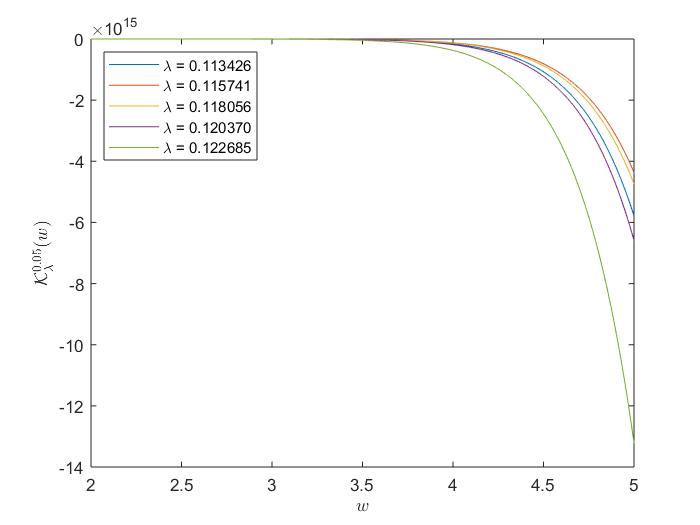
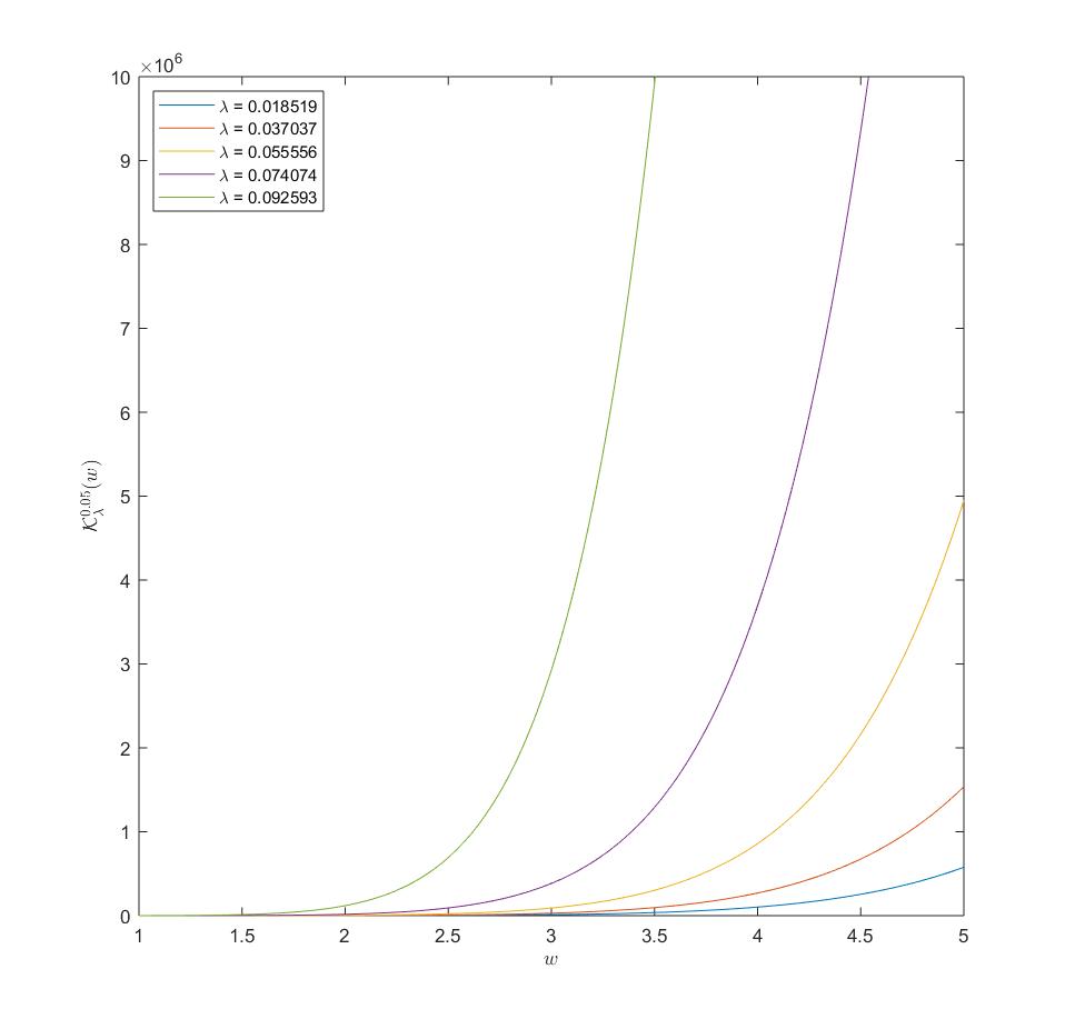
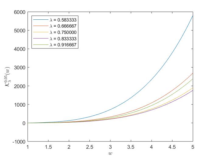
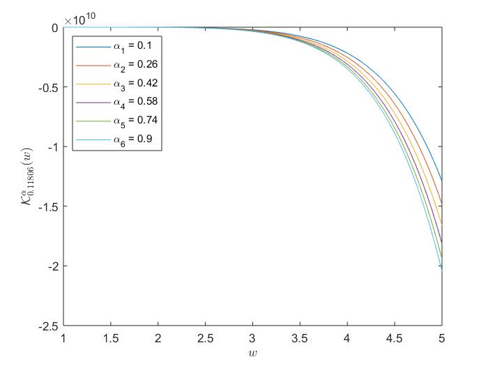
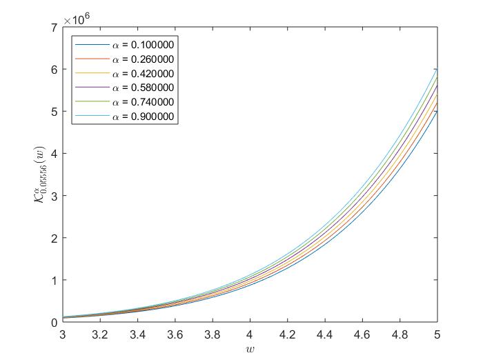
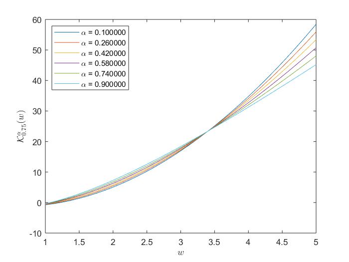
In the current section, we propose a new solution to fractional λ−kinetic equations based on generalized de-generate hypergeometric functions (GDHFs), which was further supported by graphical presentations derived through pathway-type transform approach methodologies.
Recently, Yagci and ¸Sahin [ ˘ 85] introduced the degenerate Pochhammer symbol using the degenerate Gamma function as follows:
Γλ(ϖ + ℓ) (ϖ; λ)ℓ = Γ(ϖ) Z (4.61)
− ϖ+ℓ−1
= (1 + λw) λ w dw, λ > Re(ϖ + ℓ) > 0, Γ(ϖ) 0
where λ ∈ (0, 1) and limλ→0 (ϖ; λ)ℓ = (ϖ)ℓ, is the standard Pochhammer symbol. By using (4.61), the GDHF is defined in [?] as
(γ1; λ) · · · γm ∞ λ λ (γ1; λ)r · · · (γm)r w mDHn(w) = mDHn ; w = . , (4.62) (ϑ1)r · · · (ϑn)r r!
ϑ · · · ϑ r=0
where w, γi ∈ C for i = 1, 2, 3, ..., m, and ϑj ∈ C \ Z for j = 1, 2, 3, ..., n.
• Main Results
Theorem 4.47. [89]. Let α, β, σ, ℘ ∈ R , w ∈ C, λ ∈ (0, 1), γi ∈ C for i = 1, 2, 3, ..., m and ϑj ∈ C \ Z for j = 1, 2, 3, ..., n. The solution of
λ β β α −α
K(w) − K0 mDHn(σ w ) = −℘ 0Dw K(w), (4.63)
is
X (γ ; λ) · · · (γ ) Γ(βr + 1)
α 1 r m r βr rβ α α
Kλ (w) = K0 σ w Eα,βr+1(−℘ w ), (4.64) (ϑ1)r · · · (ϑn)r r!
where Eθ,ϑ(η) is the generalized Mittag-Leffler function defined as
Eθ,ϑ(η) = (θ, ϑ ∈ C, Re(θ) > 0, Re(ϑ) > 0). (4.65) Γ(ıθ + ϑ)
A variety of special cases of this result are given in [89].
(1A)
(1B)
(1C) (2A)
(2B)
(2C)
5. Concluding Remarks and Future Works
The applications of special functions and fractional analysis theory are not restricted to the issues listed above. Recently, the study of the extension of several special functions and polynomials linked with fractional operators has gained importance. Thus, the researchers have derived several generalizations and developments of special functions and fractional calculus through various studies. From this perspective, in this review article, we offer a variety of results from these investigations.
As future work, we are, joining with others, planning to:
• Extend the results given in the above sections to quaternionic and Clifford analysis.
• Investigate the numerical methods for special matrix functions related to fractional calculus.
• The applications of analytical properties of generalized special functions of fractional calculus across different fields are studied.
References
- [1] I.N. Sneddon, Special Functions of Mathematical Physics and Chemistry. Longman Mathematical Texts, (1980).
- [2] A.F. Nikiforov, V.B. Uvarov, VUvarov, Special Functions of Mathematical Physics. A Unified Introduc-tion with Applications, 205, Springer (1988).
- [3] W.W. Bell, Special functions for scientists and engineers. Courier Corporation, (2004).
- [4] B. Dwork, Generalized hypergeometric functions. Oxford University Press, (1990).
- [5] P.J. Davis, Leonhard euler’s integral: A historical profile of the gamma function: In Memoriam: Milton Abramowitz, The American Mathematical Monthly 66:10, 849–869 (1959).
- [6] G.M. Mittag-Leffler, Sur la nouvelle fonction Eα(x), C. R. Acad. Sci. Paris, 137:2, 554–558 (1903).
- [7] H.J. Haubold, A.M. Mathai, R.K. Saxena, Mittag-Leffler functions and their applications. Journal of Applied Mathematics, 1, 298628 (2011).
- [8] M. Abdalla, Special matrix functions: characteristics, achievements and future directions. Linear and Multilinear Algebra, 68:1, 1–28 (2020).
- [9] J. Tenreiro Machado, V. Kiryakova, F. Mainardi, A poster about the old history of fractional calculus. Fractional Calculus and Applied Analysis, 13:4, 447–454 (2010).
- [10] T. Machado, V. Kiryakova, F. Mainardi, A poster about the recent history of fractional calculus. Fractional Calculus and Applied Analysis, 13:3, 329–334 (2010).
- [11] J.T. Machado, V. Kiryakova, F. Mainardi, Recent history of fractional calculus. Communications in Non-linear Science and Numerical Simulation, 16:3, 1140–1153 (2011).
- [12] V. Kiryakova, Unified approach to fractional calculus images of special functions—A survey. Mathemat-ics, 8:12, 2260 (2020).
- [13] J. Lovoie, T.J. Osler, R. Tremblay, Fractional derivatives and special functions. SIAM Review, 18:2, 240– 268 (1976).
- [14] K. Oldham, J. Spanier, The Fractional Calculus Theory and Applications of Differentiation and Integra-tion to Arbitrary Order. Elsevier, 1974.
- [15] A. Kilbas, Fractional calculus of the generalized Wright function. Fractional Calculus and Applied Anal-ysis, 8:2, 113–126 (2005).
- [16] V. Kiryakova, Some special functions related to fractional calculus and fractional (non-integer) order control systems and equations. Facta Univ. Ser. Autom. Control Robot, 7:1, 79–98 (2008).
- [17] H.M. Srivastava, Special Functions in Fractional Calculus and Related Fractional Differintegral Equa-tions. Verlag Nicht Ermittelbar, (2015).
- [18] A. Kochubei, Y. Luchko, V.E. Tarasov, I. Petráš, Handbook of Fractional Calculus with Applications, vol. 1, De Gruyter Berlin, Germany, (2019).
- [19] H. Singh, H. Srivastava, R. Pandey, Special Functions in Fractional Calculus and Engineering. CRC Press, (2023).
- [20] S. Mubeen, G. Habibullah, k-Fractional integrals and application. Int. J. Contemp. Math. Sci., 7:2, 89–94 (2012).
- [21] G. Rahman, K. S. Nisar, and S. Mubeen, On generalized k-fractional derivative operator, AIMS Mathe-matic 5 (2020), 1936-1945.
- [22] P. Agarwal, M. Chand, D. Baleanu, D. O’Regan, S. Jain, On the solutions of certain fractional kinetic equations involving k−Mittag-Leffler function. Advances in Difference Equations, 2018, 249 (2018).
- [23] M. Abdalla, S. Boulaaras, M. Akel, S.A. Idris, S. Jain, Certain fractional formulas of the extended k-hypergeometric functions. Advances in Difference Equations, 450, 450 (2021).
- [24] M. Hidan, M. Akel, H. Abd-Elmageed, and M. Abdalla, Solution of fractional kinetic equations involving extended (k, t)-Gauss hypergeometric matrix functions. AIMS Math. 7:8, 14474–14491 (2022).
- [25] O. Marichev, Volterra equation of Mellin convolution type with a Horn function in the kernel. Izvestiya Akademii Nauk SSSR. Seriya Fiziko Matematicheskikh Nauk, 1, 128–129 (1974).
- [26] M. Saigo, A remark on integral operators involving the Gauss hypergeometric functions. Math. Rep. Kyushu Univ., 11, 135–143 (1978).
- [27] M. Saigo, A certain boundary value problem for the Euler-Darboux equation. II, Math. Japon 25 (1980), 211220.
- [28] M. Saigo and N. Maeda, More generalization of fractional calculus. Transform Methods and Special Functions, Varna, Bulgaria, 386–400 (1996).
- [29] R. Saxena and M. Saigo, Generalized fractional calculus of the H-function associated with the Appell function F3. J. Fract. Calc., 19, 89–104 (2001).
- [30] H. Kober, On fractional integrals and derivatives. The Quarterly Journal of Mathematics, 11:1, 193–211 (1940).
- [31] M. Abdalla, M. Akel, Computation of Fourier transform representations involving the generalized Bessel matrix polynomials. Advances in Difference Equations, 2021, 418 (2021).
- [32] M.H. Al-Lail, A. Qadir, Fourier transform representation of the generalized hypergeometric functions with applications to the confluent and Gauss hypergeometric functions. Applied Mathematics and Computation, 263, 392–397 (2015).
- [33] Y. Luchko, Some schemata for applications of the integral transforms of mathematical physics. Mathe-matics, 7:3, 254 (2019).
- [34] V. Serov et al., Fourier Series, Fourier Transform and Their Applications to Mathematical Physics. 197, Springer, (2017).
- [35] L. Debnath, D. Bhatta, Integral Transforms and their Applications. Chapman and Hall/CRC, (2016).
- [36] B. Davies, Integral transforms and their applications. Springer Science and Business Media, 41, 2012.
- [37] M. Akel, H.M. Elshehabey, R. Ahmed, Generalized Laplace-type transform method for solving multilayer diffusion problems. Journal of Function Spaces, (2022).
- [38] M.A. Asiru, Sumudu transform and the solution of integral equations of convolution type. International Journal of Mathematical Education in Science and Technology, 32:6, 906–910 (2001).
- [39] H. Eltayeb, A. Kılıçman, On some applications of a new integral transform. International Journal of Mathematical Analysis, 4:3, 123132 (2010).
- [40] M. Ramadan, H.M. Arafa, A reliable approach of Ramadan group integral and projected differential trans-form methods to system of nonlinear partial differential equations. Filomat, 37:23, 7891–7903 (2023).
- [41] D. Kumar, Solution of fractional kinetic equation by a class of integral transform of pathway type. Journal of Mathematical Physics, 54:4, 043509 (2013)
- [42] D. Kaur, M. Chand, M. Rakshit, On pathway fractional integral formulae involving new extended hyper-geometric functions. Int. J. Manag. Technol. Eng., 9:5, 1461–1469 (2019).
- [43] D. Baleanu, P. Agarwal, A composition formula of the pathway integral transform operator. Note di Matematica, 34:2, 145–156 (2015).
- [44] R. Agarwal, M.P. Goswami, R.P. Agarwal, Hankel transform in bicomplex space and applications. TJMM, 8:1, 01–14 (2016).
- [45] T. Kumar, A. Prasad, Pseudodifferential operators involving linear canonical Hankel transformations on some ultradifferentiable function spaces. Mathematical Methods in the Applied Sciences, 44:6, 4686–4700 (2021).
- [46] N. Irfan, A. Siddiqi, et al., A wavelet algorithm for Fourier-Bessel Transform arising in optics. Int. J. Eng. Math., 9, 1–9 (2015).
- [47] V.K. Tuan, M. Saigo, et al., Convolution of Hankel transform and its application to an integral involving Bessel functions of first kind. International Journal of Mathematics and Mathematical Sciences 18, 545– 549 (1995).
- [48] E.A. Kuffi, N.K. Meftin, E.S. Abbas, E.A. Mansour, A review on the integral transforms. Eurasian Journal of Physics, Chemistry and Mathematics, 1, 20–28 (2021).
- [49] P. Agarwal, Certain properties of the generalized Gauss hypergeometric functions. Applied Mathematics and Information Sciences, 8:5, 2315 (2014).
- [50] L. Jodar, J. Cortés, On the hypergeometric matrix function. Journal of Computational and Applied Math-ematics, 99:1-2, 205–217 (1998).
- [51] H. Srivastava, Certain properties of a generalized Whittaker transform. Mathematica (Cluj), 10:33, 385– 390 (1968).
- [52] H.J. Haubold, A.M. Mathai, The fractional kinetic equation and thermonuclear functions. Astrophysics and Space Science, 273, 5363 (2000).
- [53] R. Saxena, S.L. Kalla, On the solutions of certain fractional kinetic equations. Applied Mathematics and Computation, 199:2, 504511 (2008).
- [54] R. Saxena, A. Mathai, H. Haubold, On generalized fractional kinetic equations. Physica A: Statistical Mechanics and its Applications, 344:3-4, 657–664 (2004).
- [55] R. Saxena, A. Mathai, H. Haubold, On fractional kinetic equations. Astrophysics and Space Science, 282, 281–287 (2002).
- [56] N. Virchenko, S. Kalla, A. Al-Zamel, Some results on a generalized hypergeometric function. Integral Transforms and Special Functions, 12:1, 89–100 (2001).
- [57] A. Bakhet, Y. Jiao, F. He, On the Wright hypergeometric matrix functions and their fractional calculus. Integral Transforms and Special Functions, 30:2, 138–156 (2019).
- [58] M. Abdalla, Fractional operators for the Wright hypergeometric matrix functions. Advances in Difference Equations, 1, 246 (2020).
- [59] M. Abdalla, M. Haidan, Fractional orders of the generalized Bessel matrix polynomials. European Journal of Pure and Applied Mathematics, 10:5, 995–1004 (2017).
- [60] M. Abdalla, S.A. Idris, I. Mekawy, Some results on the extended hypergeometric matrix functions and related functions. Journal of Mathematics, 1, 2046726 (2021).
- [61] B. Çekim, Generalized Euler’s beta matrix and related functions. AIP Conf. Proc., 1558, 1132–1135 (2013).
- [62] M. Abdalla and A. Bakhet, Extended Gauss hypergeometric matrix functions. Iranian Journal of Science and Technology, Transactions A: Science, 42, 1465–1470 (2018).
- [63] R. Diaz and E. Pariguan, On hypergeometric functions and Pochhammer symbol. Divulgaciones Matem-aticas, 15:2, (2005).
- [64] A. Ali, M.Z. Iqbal, T. Iqbal, M. Hadir, Study of Generalized hypergeometric functions. Computer Science, 16:1, 379–388 (2021).
- [65] M. Abdalla, M. Hidan, Investigation of the k−analogue of Gauss hypergeometric functions constructed by the Hadamard product. Symmetry, 13:4, 714 (2021).
- [66] J. Zhou, H. Li, Y. Xu, A Kummer-type transformation for some khypergeometric functions. Applicable Analysis, 101:5, 16511658 (2022).
- [67] F. He, A. Bakhet, M. Hidan, H. Abd-Elmageed, On the construction of (p, k)-hypergeometric function and applications. Fractals, 30:10, 2240261 (2022).
- [68] M. Hidan, S.M. Boulaaras, B.-B. Cherif, M. Abdalla, Further results on the ( p, k )- analogue of hyperge-ometric functions associated with fractional calculus operators. Mathematical Problems in Engineering, 1, 5535962 (2021).
- [69] M.Z. Alqarni, M. Abdalla, Analytic properties and numerical representations for constructing the extended beta function using logarithmic mean. AIMS Mathematics, 9:5, 12072–12089 (2024).
- [70] M.A. Chaudhry, A. Qadir, M. Rafique, S. Zubair, Extension of Euler’s beta function. Journal of Compu-tational and Applied Mathematics, 78:1, 19–32 (2024).
- [71] R. Mustapha, M. Chergui, On a new parameterized beta function. Proc. of the Institute of Math. and Mechanics, National Academy of Sciences of Azerbaijan, 48:1, 132–139 (2022).
- [72] M. Abdalla, Y. Almalki, I. Mekawy, and H. Abd-Elmageed, Extended Hypergeometric Logarithmic Func-tions and Its Application in Generalized Fractional Kinetic Equations, Accepted in Fractals, (2025).
- [73] E. Defez, L. Jódar, A. Law, Jacobi matrix differential equation, polynomial solutions, and their properties. Computers and Mathematics with Applications, 48:5-6, 789–803 (2004).
- [74] G.S. Kahmmash, A study of a two variables Gegenbauer matrix polynomials and second order matrix partial differential equations. Int. J. Math. Anal., 2, 807–821 (2008).
- [75] S. Khan and N. Raza, 2-variable generalized Hermite matrix polynomials and Lie algebra representation. Reports on Mathematical Physics, 66:2, 159–174 (2010).
- [76] F. He, A. Bakhet, M. Hidan, M. Abdalla, Two variables Shivley’s matrix polynomials. Symmetry, 11:2, 151 (2019).
- [77] M. Abdalla, M. Hidan, Analytical properties of the two-variables Jacobi matrix polynomials with appli-cations. Demonstratio Mathematica, 54:1, 178–188 (2021).
- [78] R. Khan, N. Kumar, R. Qamar, Two variables generalization of Jacobi polynomials. Global Journal of Pure and Applied Mathematics,13:5, 1387–1399 (2017).
- [79] M. Hidan, M. Akel, S.M. Boulaaras, M. Abdalla, On behavior Laplace integral operators with generalized Bessel matrix polynomials and related functions. Journal of Function Spaces, 10, 9967855 (2021).
- [80] M. Abdalla, On Hankel transforms of generalized Bessel matrix polynomials. AIMS Mathematics, 6:6, 6122–6139 (2021).
- [81] L. Jódar, R. Company, E. Navarro, B essel matrix functions-explicit solution of coupled Bessel type equations. Utilitas Mathematica, 46, 129–141 (1994).
- [82] M. Abdalla, S. Boulaaras, M. Akel, On Fourier-Bessel matrix transforms and applications. Mathematical Methods in the Applied Sciences 44:14, 11293–11306 (2021).
- [83] Y. Singh, V. Gill, J. Singh, D. Kumar, I. Khan, Computable generalization of fractional kinetic equation with special functions. Journal of King Saud University-Science, 33:1, 101221 (2021).
- [84] M. Abdalla, M. Akel, Contribution of using Hadamard fractional integral operator via Mellin integral transform for solving certain fractional kinetic matrix equations. Fractal and Fractional, 6:6, 305 (2022).
- [85] M. Chand, Ö. Özen, J.C. Prajapati, Solution of generalized fractional kinetic equations with generalized Mathieu series. Georgian Mathematical Journal, 31:2, 187–193 (2024).
- [86] M.Z. Alqarni, M. Akel, M. Abdalla, Solutions to fractional q-kinetic equations involving quantum exten-sions of generalized hyper Mittag-Leffler functions. Fractal and Fractional, 8:1, 58 (2024).
- [87] M. Akel, M. Hidan, S. Boulaaras, M. Abdalla, On the solutions of certain fractional kinetic matrix equa-tions involving Hadamard fractional integrals. AIMS Math., 7:8, 15520–15531 (2022).
- [88] O. Yahci and R. ¸Sahin, Degenerate Pochhammer symbol, degenerate Sumudu transform, and degenerate hypergeometric function with applications. Hacettepe Journal of Mathematics and Statistics, 50:5, 1448– 1465 (2021).
- [89] M.Z. Alqarni, M. Abdalla, Novel kinds of fractional λ-kinetic equations involving the generalized degen-erate hypergeometric functions and their solutions using the Pathway-Type integral. Mathematics, 11:19, 4217 (2023). Author information Mohamed Abdalla, Mathematics Department, Faculty of Science, South Valley University, Qena 83523, EGYPT. E-mail: mohamed.abdulah@sci.svu.edu.eg, moabdalla@kku.edu.sa Received: 01.08.2024 Accepted: 05.11.2024 Published: 27.12.2024